Data Mining: Bagging and Boosting Increasing Classification ...

Increasing Classification Accuracy

Data Mining: Bagging and Boosting Andrew Kusiak Intelligent Systems Laboratory 2139 Seamans Center The University of Iowa Iowa City, Iowa 52242 - 1527

‰ Bagging gg g ‰ Boosting ‰ Meta-learning (stacking)

[email protected] http://www.icaen.uiowa.edu/~ankusiak Tel: 319 - 335 5934 The University of Iowa

Intelligent Systems Laboratory

The University of Iowa

Intelligent Systems Laboratory

Bagging 2

Bagging 1 Sample 1

Learning algorithm

Classifier 1

Corporate decision-making analogy ƒ Managers g seeks advice of experts p in areas that s/he does not have expertise ƒ The skills of the advisers should complement each other rather than being duplicative

New data

Training g data

Sample p 2

Learning algorithm

Sample 3

Learning algorithm

Classifier 2

Bootstrap scheme

Combined classifier

Predicted decision

Voting scheme Classifier 3

Applies also to boosting (1 - 1/n)n ~ e-1 = .368, where e = 2.7183 The University of Iowa

Intelligent Systems Laboratory

The University of Iowa

Intelligent Systems Laboratory

1

Bagging 3

Bagging 4

Bagging Procedure Classifier generation Step 1. Create t data sets from a database applying the sampling with replacement scheme. Step 2. 2 Apply a learning algorithm to each sample training data set. Classification Step 3. For an object with unknown decision, make predictions with each of the t classifiers. Step 4. Select the most frequently predicted decision. The University of Iowa

Intelligent Systems Laboratory

• Classification – Voting scheme • Prediction – Averaging scheme • Also used – Bagging with costs and randomization schemes within learning algorithms (e.g., features with equal value gain) The University of Iowa

Bagging 5

Boosting 1

• The effect of combining different classifiers (hypotheses) can be explained with the theory of bias-variance decomposition • Bias – an error due to a learning algorithm • Variance – an error due to the learned model (data set related) • The total expected error of a classifier = Bias + Variance The University of Iowa

Intelligent Systems Laboratory

Intelligent Systems Laboratory

• Bagging – Individual models are built separately • Boosting – Combines models of the same type (e.g., decision tree) and it is iterative, i.e., a new model is influenced by the performance of the previously built model • Boosting – Uses voting or averaging (similar to bagging) • Different boosting algorithms exist The University of Iowa

Intelligent Systems Laboratory

2

Boosting 3 Boosting 2 • Method – AdaBoost.M1 which is widely used • Assumption: Learning algorithm can handle weighted instances (usually handled by randomization schemes for selection of training data subsets) • By weighting instances, the learning algorithm can concentrate on instances with high weights (called “hard” instances), i.e., incorrectly classified instances The University of Iowa

Intelligent Systems Laboratory

AdaBoost.M1 Algorithm (Outline) • All instances are equally weighted • A learning algorithm is applied • The weight of incorrectly classified examples is increased (“hard” instances), correctly – decreased (“easy” ( easy instances) • The algorithm concentrates on incorrectly classified “hard” instances • Some “had” instances become “harder” some “softer” • A series of diverse experts (classifiers) is generated based on the reweighed data The University of Iowa

Boosting 4

Intelligent Systems Laboratory

Boosting 4

AdaBoost.M1 Algorithm (Steps) Classifier generation Step 0. Set the weight value, w = 1, and assign it to each object in the training data set. For each of t iterations, perform: Step 1. Apply a learning algorithm to the weighted training data set. Step 2. Compute classification error e for the weighted training data set. If e = 0 or e >=.5, then terminate the classifier generation process and go to Step 4; otherwise multiple the weight w of each object by e/(1 – e) and normalize the weights of all objects.

Classification Step 4. Assign weight q = 0 to each decision (class) to be predicted. Step 5. For each of t (or less) classifiers, add –log e/(1 – e) to the weight of the decision predicted by the classifier and output the decision with the highest weight. The University of Iowa

Intelligent Systems Laboratory

For e = 0 all training examples (objects) are correctly classified (a perfect classifier) and therefore there is no reason to modify the object weights, i.e., for e/(1 – e) = 0 all new weights w become 0.

For e = .5, the expression – log e/(1 – e) = 0, and therefore the weights q = 0 are not be modified and therefore no decision is generated due to high classification error e.

The University of Iowa

Intelligent Systems Laboratory

3

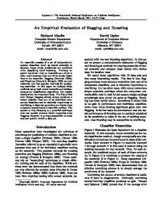
Meta-learning Learning algorithm 1

Training data

Creating Meta-training Data ‰ Voting Each classifier gets one vote and the majority wins.

Classifier 1

‰ Weighted voting Provides preferential treatment to some voting classifiers.

Test data Learning algorithm l ih 2

Trainingg data

Classifier 2 Predicted decisions

Metaclassifier

Predicted decisions

The University of Iowa

Metalearning algorithm

Predicted decisions

Metatraining data

Intelligent Systems Laboratory

‰ Arbitration An arbitrator makes a selection, if the classifiers can not reach a consensus. ‰ Combining Decisions produced by different classifiers are combined as one decision. The University of Iowa

Intelligent Systems Laboratory

Example (2) Example (1) Object No.

Features

Decision

1

Vector 1

High

2

Vector 2

Low

3

Vector 3

High

The University of Iowa

Intelligent Systems Laboratory

Object No. 1 2 3

Features Vector 1 Vector 2 Vector 3

Decision High Low High

Predictions of classifiers 1 and 2 for the training data set Object No. Classifier 1 Prediction

Classifier 2 Prediction

1

High

High

2

High

Low

3

Low

Low

The University of Iowa

Intelligent Systems Laboratory

4

Example (4)

Example (3)

Object No. Classifier 1 Prediction Classifier 2 Prediction

Object No. Classifier 1 Prediction Classifier 2 Prediction 1 2 3

High High Low

High

1

High

Low

2

High

Low

Low

3

Low

Low

Training set generated by the class-attribute-combiner scheme

Training g set generated g byy the class-combiner scheme Object No.

Features

Decision

1

High, High

High

2

High, Low

Low

3

Low, Low

High

The University of Iowa

High

Intelligent Systems Laboratory

Object No.

Features

Decision

1

High, High, Vector 1

High

2

High, Low, Vector 2

Low

3

Low, Low, Vector 3

High

The University of Iowa

Example (5)

Intelligent Systems Laboratory

Example (6)

Object No. Classifier 1 Prediction Classifier 2 Prediction 1

High

2

High

High Low

3

Low

Low

Binary form of the predictions produced by classifier 1 Object No. Classifier 1 Prediction Feature = High

T i i set generatedd by Training b the h binary bi class-attribute-combiner l ib bi scheme h Object No.

The University of Iowa

Feature Vector

Decision

1

Yes, No, Yes, No

High

2

Yes, No, No, Yes

Low

3

No ,Yes, No, Yes

High

Intelligent Systems Laboratory

Feature = Low

Decision

1

High

Yes

No

High

2

High

Yes

No

Low

3

Low

No

Yes

High

The University of Iowa

Intelligent Systems Laboratory

5

Meta-learners

Distributed Learning

‰ Integration of knowledge learned from different and distributed databases. ‰ Elimination of inductive bias. ‰ Extraction of high level models. ‰ Scalability to hierarchical meta-learning.

The University of Iowa

Intelligent Systems Laboratory

Data Populations

• Distributed by partitioning • Distributed by nature

The University of Iowa

Learning from homogeneously distributed data sets Θi = Θj = Θ

• Homogeneous (Θi = Θj , i ≠ j - all learners share the same distribution) • Heterogeneous (Θi ≠ Θj , i ≠ j)

The University of Iowa

Intelligent Systems Laboratory

Intelligent Systems Laboratory

P(D|Θ)

The University of Iowa

L-learner 1

^ Θ 1

L learner 2 L-learner

^ Θ 2

L-learner n

^ Θ n

M-learner

^ Θ

Intelligent Systems Laboratory

6

Θi ≠ Θj

Learning from heterogeneously distributed data sets P(D 1| Θ 1)

L-learner 1

^t Θ 1

P(D2 | Θ2)

L-learner 2

^t Θ 2

P(Dn | Θn)

L-learner n

^t Θ n

^ μ

Gini Index 1

t

M-learner

^ μ) ^ (Θ,

• S = data set with n objects • c = number of classes in S • pj = relative frequency of class j in S c

t = step number μ models interrelationships between distributions of the local data The University of Iowa

Intelligent Systems Laboratory

gini (S) = 1 – Σ pj2 j=1

The University of Iowa

Intelligent Systems Laboratory

Gini Index 2 • • • • •

S1 = partition 1 of S n1 = number of objects in S1 S2 = partition 2 of S n2 = number of objects in S2, where n2 = (n - n1) a = splitting criterion gini (S, a) = n1/n gini (S1) + n2/n gini (S2) The University of Iowa

Intelligent Systems Laboratory

7