A TIMECENTER Technical Report. T ... optimization and processing, as well as extend the query language itself. ... Heuristics are used to reduce the search space, e.g., one heuristic is that the optimizer should consider .... Figure 2 describes the main function of the Execution Engine, which receives an execution-ready plan ...
Adaptable Query Optimization and Evaluation in Temporal Middleware
Giedrius Slivinskas, Christian S. Jensen, and Richard T. Snodgrass
TR-56
A T IME C ENTER Technical Report
�� ��� �
Adaptable Query Optimization and Evaluation in Temporal Middleware
�
� � �� �������� �� �� ��� �������� !#"$���%�& ��(' )
*
IME ENTER
Copyright c 2001 Giedrius Slivinskas, Christian S. Jensen, and Richard T. Snodgrass. All rights reserved. Giedrius Slivinskas, Christian S. Jensen, and Richard T. Snodgrass March 2001. A T IME C ENTER Technical Report.
� �+�(�����,�.-,�/0�%�
Aalborg University, Denmark Christian S. Jensen (codirector), Michael H. B¨ohlen, Heidi Gregersen, Dieter Pfoser, ˇ Simonas Saltenis, Janne Skyt, Giedrius Slivinskas, Kristian Torp University of Arizona, USA Richard T. Snodgrass (codirector), Bongki Moon Individual participants Curtis E. Dyreson, Bond University, Australia Fabio Grandi, University of Bologna, Italy Nick Kline, Microsoft, USA Gerhard Knolmayer, Universty of Bern, Switzerland Thomas Myrach, Universty of Bern, Switzerland Kwang W. Nam, Chungbuk National University, Korea Mario A. Nascimento, University of Alberta, Canada John F. Roddick, University of South Australia, Australia Keun H. Ryu, Chungbuk National University, Korea Michael D. Soo, amazon.com, USA Andreas Steiner, TimeConsult, Switzerland Vassilis Tsotras, University of California, Riverside, USA Jef Wijsen, University of Mons-Hainaut, Belgium Carlo Zaniolo, University of California, Los Angeles, USA For additional information, see The T IME C ENTER Homepage: URL:
Any software made available via T IME C ENTER is provided “as is” and without any express or implied warranties, including, without limitation, the implied warranty of merchantability and fitness for a particular purpose.
The T IME C ENTER icon on the cover combines two “arrows.” These “arrows” are letters in the so-called Rune alphabet used one millennium ago by the Vikings, as well as by their precedessors and successors. The Rune alphabet (second phase) has 16 letters, all of which have angular shapes and lack horizontal lines because the primary storage medium was wood. Runes may also be found on jewelry, tools, and weapons and were perceived by many as having magic, hidden powers. The two Rune arrows in the icon denote “T” and “C,” respectively.
Abstract Time-referenced data are pervasive in most real-world databases. Recent advances in temporal query languages show that such database applications may benefit substantially from built-in temporal support in the DBMS. To achieve this, temporal query optimization and evaluation mechanisms must be provided, either within the DBMS proper or as a source level translation from temporal queries to conventional SQL. This paper proposes a new approach: using a middleware component on top of a conventional DBMS. This component accepts temporal SQL statements and produces a corresponding query plan consisting of algebraic as well as regular SQL parts. The algebraic parts are processed by the middleware, while the SQL parts are processed by the DBMS. The middleware uses performance feedback from the DBMS to adapt its partitioning of subsequent queries into middleware and DBMS parts. The paper describes the architecture and implementation of the temporal middleware component, termed TANGO, which is based on the Volcano extensible query optimizer and the XXL query processing library. Experiments with the system demonstrate the utility of the middleware‘s internal processing capability and its cost-based mechanism for apportioning the processing between the middleware and the underlying DBMS.
Index terms: temporal databases, query processing and optimization, cost-based optimization, middleware
1 Introduction In this paper we propose a new approach, that of temporal middleware, to evaluating temporal queries that enables significant performance benefits. Most real-world database applications rely on time-referenced data. For example, time-referenced data is used in financial, medical, and travel applications. Being time-variant is even one of Inmon’s defining properties of a data warehouse [Inm96]. Recent advances in temporal query languages [EJS98, JS99] show that such applications may benefit substantially from running on a DBMS with built-in temporal support. The potential benefits are several: application code is simplified and more easily maintainable, thereby increasing programmer productivity [Sno99], and more data processing can be moved from applications to the DBMS, potentially leading to better performance. In contrast, the built-in temporal support offered by current database products is limited to predefined timerelated data types, e.g., the Informix TimeSeries Datablade and the Oracle8 TimeSeries cartridge, and extensibility facilities that enable the user to define new, e.g., temporal, data types [YYW00]. However, temporal support is needed that goes beyond data types. The temporal support should encapsulate temporal operations in query optimization and processing, as well as extend the query language itself. Developing a DBMS with built-in temporal support from scratch is a daunting task that may, at best, only be feasible by DBMS vendors that already have a code base to modify and have large resources available. This has led to the consideration of a layered, or stratum, approach where a layer that implements temporal support is interposed between the user applications and a conventional DBMS [Boe95, TJS97, TJS00, VLG98]. The stratum maps temporal SQL statements to regular SQL statements and passes them to the DBMS, which remains unaltered. A stratum approach presents difficulties of its own. First, every temporal query must be expressible in the conventional SQL supported by the underlying DBMS, which constrains the temporal constructs that can be supported. Even more problematic is that some temporal constructs, such as temporal aggregation, are quite inefficient when evaluated using SQL, but can be evaluated efficiently with application code that uses a cursor to access the underlying data. This paper proposes a generalization of the stratum approach, moving some of the query evaluation into the stratum. We term this the “temporal middleware” approach. All previous approaches have consisted entirely of a temporal-SQL-to-SQL translation, effectively a smart macro processor, with all of the work done in the DBMS, and little flexibility in the SQL that is generated. Our middleware approach, in addition to mapping temporal SQL to conventional SQL, performs query optimization and some processing. Moving some of the query processing to the middleware improves query performance because complex operations such as temporal aggregation or temporal duplicate elimination have efficient algorithms in the middleware, but are difficult to process efficiently in conventional DBMSs. Allowing some of the query processing to occur in the middleware raises the issue of deciding which portion(s) of a query to execute in the underlying DBMS, and which to execute in the middleware itself. Two transfer �� and �� , are used to move a relation from the DBMS to the middleware and vice versa. A query operations, 1
plan consists of those portion(s) to be evaluated in the middleware and SQL code for the portion(s) of the query to be processed by the DBMS. To flexibly divide the processing between the middleware and the DBMS, the middleware includes a query optimizer. Heuristics are used to reduce the search space, e.g., one heuristic is that the optimizer should consider evaluating in the middleware only those operations that may be processed more efficiently there. Costing is used to determine where to process certain operations, which is not always obvious. For example, whether to process a temporal join in the middleware or in the DBMS depends on the statistics of the argument relations, which are fed into the cost formulas. This paper makes several contributions. It validates the proposed temporal middleware architecture with an implementation that extends the Volcano query optimizer [GM93] and the XXL query processing system [BDS00]. The middleware query optimization and processing mechanisms explicitly address duplicates and order in a consistent manner. We provide heuristics, cost formulas, and selectivity estimation methods for temporal operators (using available DBMS statistics); and to divide the processing between the middleware and the DBMS, we use the above-mentioned transfer operators. Performance experiments with the system demonstrate that adding query processing capabilities to the middleware significantly improves the overall query performance. In addition, we show that the cost-based optimization is effective in dividing the processing between the middleware and the DBMS. Thereby, the proposed middleware system captures the functionality of previously proposed stratum approaches and is more flexible. The presented temporal operators, their algorithms, cost formulas, transformation rules, and statistics-derivation techniques may also be used when implementing a stand-alone temporal DBMS. This makes the presented implementation applicable to both the integrated and the layered architecture of a temporal DBMS, in turn making it relevant for DBMS vendors planning to incorporate temporal features into their products, as well as to third-party developers that want to implement temporal support. Section 2 presents the architecture of the temporal middleware, and shows how queries flow through the system. The following section presents temporal operators, their implementations in the middleware and the DBMS, and the corresponding cost formulas. For each temporal operation, we propose a method for estimating its selectivity using standard DBMS-maintainable statistics on base relations and attributes. This is needed because standard selectivity estimation does not work well for temporal operations, as we show. Section 4 explains the transformation rules and heuristics used by the middleware optimizer. Performance experiments demonstrate the utility of the shared query processing, as well as of the cost-based optimization.
2 Temporal Middleware We first present the architecture of the temporal middleware, termed TANGO (Temporal Adaptive Next-Generation query Optimizer and processor). Then follows an example of how a query is processed.
2.1 System Architecture Figure 1 shows TANGO’s architecture. The parser translates a temporal-SQL query to an algebra expression, the initial query plan, which is passed on to the optimizer. This plan assigns all processing to the DBMS and specifies � operation at the end. that the result is to be transferred to the middleware, by placing a Optimization occurs in two phases. Initially, a set of candidate algebraic query plans is produced by means of the optimizer’s transformation rules and heuristics. Next, the optimizer considers in more detail each of these plans. For each algebraic operation in a plan, it assumes that each of the algorithms available for computing that operation is being used, and it estimates the consequent cost of computing the query. This way, one best physical query execution plan, where all operations are specified by algorithms, is found for each original candidate plan. To enable this procedure, the Statistics Collector component obtains statistics on base relations and attributes from the DBMS catalog and provides them to the optimizer. The Cost Estimator component determines cost factors for the cost formulas used by the optimizer. Of the plans generated, the one with the best estimated performance is chosen for execution. The Translator-To-SQL component translates those parts of the chosen plan that occur in the DBMS into �� s that either reach the leaf level or �� s), and passes the execution-ready plan to the SQL (i.e., parts below � operator results in an SQL SELECT statement being issued, Execution Engine, which executes the plan. The
2
USER APPLICATION Temporal Query
Parser Initial Query Plan [algebra operators]
Result
Optimizer Query Plan [algorithms] Statistics
Translator To SQL
Cost Factors
Statistics Collector
Query Plan [algorithms and SQL]
Execution Engine
Cost Estimator
Data, Load Instructions SQL
Statistics
Data Loader
SQL
Run times
Data
SQL
Results
DBMS
�� while the
Figure 1: Middleware Architecture
operator results in an SQL CREATE TABLE statement being issued, followed by the invocation of a DBMS-specific data loader. Although both heuristic- and cost-based, this optimizer is lighter weight than a full-blown DBMS optimizer [Jar84, Ioa96], because less information is available to it. While the middleware treats the underlying DBMS as a (quite full featured!) file system, it is not possible for the middleware to accurately estimate the time for the DBMS to deliver a block of tuples from a perhaps involved SQL statement associated with a cursor. This contrasts with a DBMS, which can estimate the time to read a block from disk quite accurately. However, the job of a middleware optimizer is also simpler, in that it does not need to choose among a variety of query plans for the portion of the query to be evaluated by the DBMS. Rather, it just needs to determine where the processing of each part of the query should reside. It does so by appropriately inserting transfer operations into query plans. The optimizer component is an extended version of McKenna and Graefe’s Volcano optimizer [GM93], implemented in C/C++. This optimizer has been enhanced to systematically capture duplicates and order, as well as to support several different kinds of equivalences among relational expressions (e.g., equivalences that consider relations as multisets or lists) [SJS00]. The Execution Engine module is implemented in Java, uses the XXL library of query processing algorithms developed by van den Bercken et al. [BDS00], and accesses the DBMS using a JDBC interface. Figure 2 describes the main function of the Execution Engine, which receives an execution-ready plan consisting of a sequence of algorithms with their parameters and arguments. For example, an algorithm implementing temporal aggregation takes grouping attributes and aggregate functions as parameters, and a relation as its argu� takes an SQL query as its parameter. ment, while an algorithm implementing
3
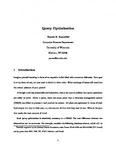
�������� ��� ������� (Query Plan ��� ): �����������! "#��$&% �� �'(� )+*#���-,/.10(2 %�3 ��45 �67)98 �#:#;/� � size b �c[�Jdfe=g Q size b �c (' * c�# � size b �Uc[��dfe=g Q size b �c cost bz�] a b �c�c>� cost b � �#� �(��KWf b �c�c�� 9hTi�' lm �9������5�UDb �c m
cost b ��fjZ� [k ��KWf [% b �c�c��
n
�p q�'sr �;�� U��^�_� ��5^�aT� b t]%Wb �c�c uTv>w U �3�xP� -a �-_��� eih�b1k�PE� c �p q�'�y �;��U
� � ^�_� �5� ^�aT � b t]W % b � c�c z]{�|/}9~� uT }
mmo
Figure 6: Cost Formulas
3.2 Transfer Operators
��
The operator transfers a relation from the DBMS to the middleware. Its implementation, the �Wf �� algorithm, is straightforward: it sends an SQL query to the DBMS via the JDBC interface and fetches result tuples. The performance of this operator depends on the number and size of the tuples transferred. Experiments with Oracle show that the performance is also affected by the row-prefetch setting, which specifies the number of
7
tuples fetched at a time by JDBC to a client-side buffer. We have not included this latter setting in our cost formula because it � is DBMS-specific. The operation transfers data from the middleware to the DBMS. Its algorithm, p Wf �� , first creates a table in the DBMS and then loads data into it. The data load is specific to the DBMS. For example, the program SQL Loader may be used in Oracle. This program needs a data file with the� actual tuples and a control file operation could use a sequence specifying the structure of the data file. An alternative implementation of the of INSERT statements; this solution would be inefficient for large amounts of data. In Oracle, a number of optimization techniques can be used to speed up the load time of SQL Loader and to minimize the size of the result table. First, direct-path load can be used (which loads data directly into the database as opposed to conventional-path load which uses INSERT statements). Second, since the size of the data to load is known, the initial memory extent allocated for the table can be equal to that size, avoiding the cost of multiple memory allocations. In addition, blocks of the new table do not have to contain any free space because the table will never be updated. The cost of p Wf �� g depends on the number and size of the tuples transferred. The name of the table created must be unique, and the table must be dropped at the end of the query.
3.3 Selection Although DBMSs have efficient selection algorithms, we have also implemented a selection algorithm in the middleware ( ��� �]� g ) because it is sometimes needed. For example, if there is a selection between two temporal algorithms to be performed in the middleware, it would be inefficient to transfer the intermediate result to the DBMS solely for the purpose of selection. The cost of ��� � ] depends on the relation size as well as on the selection predicate. Minimum and maximum values of each selection-result attribute are always the same as those of the argument attributes, unless the attribute is involved in the selection predicate so that the predicate forces the minimum value to be increased or the maximum value to be decreased. For example, predicate ( s ) leads to a (new) maximum value that is the minimum of s and the old maximum value. The number of distinct values for a result attribute is equal to the number of equality conditions on the attribute (if there are any), to the old value minus the number of “not equals” conditions on the attribute (if there are any), or is otherwise equal to the old value multiplied by the selectivity of the selection predicate. For example, if the � predicate is ( � s l ), the number of distinct values in the result is 2. If the selection predicate is non-temporal, the cardinality of the result relation is estimated using standard methods, as in current DBMSs, by either assuming a uniform distribution between the minimum and maximum values or by using histograms and assuming a uniform distribution within each histogram bucket. (A histogram divides attribute values into buckets; each bucket is assigned to a range of attribute values and stores how many attribute values fall within that range.) Standard estimation techniques are not directly suitable for temporal predicates. Current DBMSs treat time attributes as any other attributes, storing the same statistics. Straightforward use of these statistics leads to very inaccurate estimates of selections having temporal predicates. However, the statistics available from the DBMS are sufficient to adequately estimate the selectivities of such queries. We elaborate on these points next. Consider a temporal relation of 100,000 tuples, where the duration of each time period is 7 days and where time periods are uniformly distributed over the period from January 1, 1995 to January 1, 2000. Consequently, the time period start (o r ) values are between January 1, 1995 and December 25, 1999, and the time period end (oHs ) values are between January 8, 1995 and January 1, 2000. Both o r and oHs may have 1819 distinct values (the number of days between their minimum and maximum values). Each day then has about 383 tuples with an intersecting time period. Now consider a query that retrieves all tuples overlapping with the period starting on February 1, 1997 and ending on February 8, 1997 (the predicate would be UeOI�� ���Pb 1997-02-01 P 1997-02-08c ; and its SQL condition may be written as o r 1997-02-08 qPo�s 1997-02-01). Since the distribution of time periods is uniform, histograms are not needed. The number of tuples in the result should be between 383 and 383 � 2 tuples, which is about 0.4%–0.8% of the original relation. To estimate the selectivity of this query, each predicate is analyzed in turn. The first predicate results in 769/1819 = 42.3% of the original relation, and the second predicate, when applied to the result of the first selection,
�� ��
��
�� �� ����
�
�
8
results in 1064/1819 = 58.5% of the second relation, which is 24.7% of the tuples of the original relation. This is a factor of 40 too high! As an alternative to this straightforward estimation, we propose to simply take into account that the end time of a period never precedes its start time, which is a simple application of semantic query optimization. The result cardinality for the above-mentioned query can then be estimated by subtracting 9_�� e��O�eHb A r P��Uc , the number of tuples ending before or at (here, February 1, 1997), from �as U-a e��OU�ePb��(PE�c , the number of tuples starting before � (here, February 8, 1997). Functions pa+ -a e��OU�ePb P��c and L_�� e��OU�eHb PE�c , where is a time-attribute value in relation � , are defined next. Their definitions depend on whether histograms on o r and oHs are available. For a given histogram � , functions ���Kb� 5P � c and � �(b� �P � c return the start and end values of bucket ; function ���� ��zb� �P � c returns the number of attribute values in the -th bucket, and function �ifg�b P��Hc return the number of buckets to which attribute value belongs. 6 � 1 %!32.�� 5�����7��0� � ��������"!#�� %$�&:���0�$#&%(' ��8924�� 5�����7���� � 1 %!�24�� @�����7����"!
��� ��
1 ��
�
-.$@����$��?+��; ���+F��6.7������
� ��
*�+-,/./*�021�35476 8�. 9;:�< 6?G � �A@9����B
���
:��64/7 ��*��7/�?�� �.24�� ����B .��6.7;��*��7/����ED�FHG2IKJALM#�N7I � CE����B .��647/��*��7/�?�� �C�A@9����B .��6.7/�?���7/��*� ! ��� ��
1 ��
O
�
!:�A�?+��� ���+���6.7������
�����7����
�.2.�� ��=�7/��*���/> )
��
< ���>= %��$@ �A��>� 1
� �� �� ���
6�� 1 %!32.�� 5���KPF7��0� ��������"!#�� %$�&:���0�$#&%(' ��8924�� 5���KP 7�� � � � 1 %!�24�� @���KP 7����"! )
< ���>= %��$@ �A��>� 1
���KP 7����
�.2.�� ��=�7/�KP0���/>
*�+-,/./*�021�35476 8�. 9�QR< 6?G � �A@9����B
:��64/7 �KP0��7/�SP�� �.24�� ����B .��6.7;�KP0��7/�KP��ED�FHG2IKJALM#�N7I � CE����B .��647/�KP0��7/�SP�� �C�A@9����B .��6.7/�SP���7/�KP0� !
To compute these functions using histograms, we find the bucket containing attribute value . Then we sum the number of values in all preceding buckets and add a fraction of the number of values in the bucket containing , assuming a uniform distribution of the values within the bucket. The formulas are valid for both height-balanced histograms (where each bucket has the same number of values) and width-balanced histograms (where each bucket is of the same length); functions ���Fb� �P � c , � � b� �P � c , ���] \�zb� �P � c would return different values for different types of � . For the given query, 9_�� e��OU�e�b 1997-02-02P c is 769/1819 = 42.3% of the original relation, and �as U-a e��O�ePb 1997-02-08P c is 755/1819 = 41.5% of the original relation, leading to an estimated size of the result of 0.8% of the original relation, which is close to the actual result. For a timeslice predicate—such as (o r$T ) which returns all tuples with time periods containing qP o�s time point —the result cardinality is �as U-a e��OUiePb A r PE�cVU 9_�� e��O�e�b A r PE�c . The proposed estimation technique has some resemblance to a previous proposal [SS00], which uses two temporal histograms: one for the starting points of time periods, and one for “active” time periods (a time period is active during a histogram bucket time period . if it starts before . and overlaps with . ). The second histogram is not available from current DBMSs. In contrast, we use only statistics maintained by current DBMSs. The formula for Ue�I�� 5�pDb P���c without histograms follows the estimation techniques given in [GS90].
3.4 Temporal Join � ���
Temporal join ( ) joins tuples that have equal join attributes and overlapping time periods. Time attributes o r and o�s contain the intersection period in the result. DBMSs have efficient join algorithms, but there are cases when temporal join can be performed more efficiently in the middleware. We consider a straightforward temporal join algorithm, � p���f , which takes two relations sorted on the join attribute and merges them, comparing the time-attribute values. More efficient algorithms could be used [SSJ94], but the current algorithm is sufficient to illustrate the functioning of TANGO. The cost formula for the algorithm is given in Figure 6. In the DBMS, temporal join is implemented by regular join, selection, and projection (see Section 3.6). When estimating the selectivity of a temporal join, we use the following assumptions: the lifespans of relations to be joined are identical, the values of join attributes are uniformly distributed, the time periods for these values 9
are uniformly distributed throughout the entire lifespan, and there is a referential integrity constraint on the values (for each join-attribute value of the referenced relation, there is a corresponding value in the referencing relation). � � � With these assumptions, we derive that the cardinality of � O K5M 2*U K5M N � Q is
����
�
�
b5�U^M-a#^�_��Oa7b����
� �e�I�� ��=�p^�_Pd �
����
O�P��-OOc�P��^M-a#^�_��Oa�b 9Q=PE��Q c�c3��
eO-^1���1P
���
���
where UeOI�f 5�=�^�_Dd e�-^1��U is the number of overlapping periods for each pair of equal values of �O and ;Q . � We also derive that the minimum and maximum bound, respectively, of Ue�I�� 5� �p^�_Dd e�-^1��U is
�
b �U��^M -�a�^��U_�^�_���a� �b��Q��^�a�� � O�b P�� �-O O�c c P ���^M U-�a#^��_�^�_��Oa
\b��Q��^�aT�;� Q\ b PE� ��Q Q c c c
and
��
�U � ^�_� ��Q^�a�� b � O c A �U^M-a�^�_���a�b O-P��-O7c
����
��U
� � ^�_� ��5^�aT� b � Q c �^Mwa�^�_���a7b 9Q=PE��Q c
� ��
����
U
Since, in experiments, we use data with irregularly occurring updates, we chose to use the minimum bound plus 80% of the difference between the maximum and minimum bounds. The selectivity estimation technique used corresponds to the one presented in [Seg93].
3.5 Temporal Aggregation � �
Temporal aggregation ( ) is one of those operators that clearly benefit from running in the middleware versus in the DBMS. We have implemented a middleware implementation, Dj] , and a DBMS implementation, Dj]g , which is a 50-line SQL query. Figure 7(a) gives an example of temporal aggregation SQL query computing the �l �qPo aggregate for the k�lDm�n�onl�q relation. While it is possible to write this query in a more compact way (in about 25 lines, using views), to our knowledge, the provided code yields the best performance 1. Below we discuss Dj]j as well as how the result cardinality is derived. For /j ]g , we require its argument to be sorted on the grouping attribute values and on o r , because if tuples of the same group are scattered throughout the relation, aggregate computation requires scanning of the whole relation for each group. Meanwhile, if the argument is ordered on the grouping attributes, only a certain part of the argument relation is needed at a time. The sorting enables reading each tuple only once. In addition, another copy of the argument is sorted on all grouping attributes and o�s . The first sorting is performed by an external algorithm ( �] or F] ), while the second sorting is performed internally by the Dj]g algorithm. The algorithm traverses both copies of the argument similarly to sort-merge join and computes the aggregate values group by group. Figure 7(b) outlines its pseudo-code for computing the �l �qPo aggregate; the code has to be modified slightly for computing other aggregates. The algorithm is different from the temporal aggregation algorithms presented in [KS95], which used aggregation trees in memory or, during computation, maintained lists of constant periods and their running aggregate values. The cost of temporal aggregation in the middleware depends on the size of the argument and of the result (see Figure 6). For simplicity, the complexity of the actual aggregate functions (such as n�q or ) is not included, but experiments show that different such functions do not change the cost significantly. The cost of internal sorting is accounted for. � � The upper bound for the cardinality of 0/2I4767676 4 0"894 :92�4767676 4 :=< b �c is �� U5�U^�_� \�Q^�a��b �cX� U , and the lower bound (for a non-empty relation) is . Knowing the number of distinct values for the grouping and the time attributes allows us to tighten the range between the minimum and maximum. The minimum cardinality is b5�U^M-a#^�_��Oa7b O\PE�c�P �P;�U^M-a#^�_��Oa7b (P��Uc�P��^M-a#^�_��Oa�b1o r\P��Uc]A =P;�U^M-a�^�_���a�b o�sXPE�cXA
c . If there are no grouping attributes, the maximum cardinality is �U^M-a#^�_��Oa b o r=PE�c/A �^M-a#^�_��Oa�b1o�s P��Uc3A . Otherwise, it is
� ��
� ��
�
b
����
�� �
����
��
���� �
���!
"
#
$&%('�) �U^M-a�^�_���a���b� U� 5O\�UPE^�_��c \47�Q67^�67a�6 4 ��Ub ^M�-a#c ^�_��Oa7b���!(P��Uc(* �+� �
c/� , � b��U^M-a�^�_���a�b�� O\PE�c�P�� ����P-�U^M-a�^�_���a�b���!�P��UcicIP $U
where the fraction represents the average number of tuples for each value of the grouping attribute having the most distinct values, and the factor to the right represents the maximum number of the resulting time periods for each such value. We multiply it by the maximum number of distinct values for the grouping attributes. For experiments, we use 60% of the maximum cardinality if the resulting value is bigger than the minimum cardinality, and the minimum cardinality, otherwise. 1 Incidentally,
this SQL query may be formulated as of the existing temporal SQLs.
-y
vw!"-Owy t�|O}�x�~
10
,
Ou�O{-y (t�|O}�x�~
)
�
� u�� t�uwv xzy�x�ui{ ��� u�Ot
�
t�|O}�x�~
in one
vw!"-Owy� .t�|O}�x�~ , .y� , .yO
, Ou�O{-y ( .t�|O}�x�~ ) � �u �(t�uwv xzy�x�ui{� , vw!"-OwyF�y �Ot� .t�|O}�x�~ , y��Ot� .y� Ov y� , y��OtO
.yO
�OvKyO
( � � � u �Ft�uwv xzy�x�ui{F�y �Ot� , t�uwv xzy�x�ui{(y��OtO
���O � �� y �Ot� t�|O}�x�~ �y �OtO
t�|O}�x�~ -{w~F�y �Ot� ..y� $ �y �O=tO
.yO
. -{w~F{�uiyK� �x�vwyOv vw!"-Owy * ( � � � u �(t�uwv xzy�x�ui{��y �O�t � ���O � F� y �Ot� t�|O}�x�~ �y �O�t � t�|O}�x�~ -{w~ ((�y �Ot�. .y� $ =�y �O�t � .y�. -{w~(�y �O�t � .y� $ �y �OtO
.yO
) u � �y �Ot� y� $ �y �O�t � .yO
�-{w~��y �O�t � .yO
$ �y �OtO
.yO
))) O{�x�ui{ ( . vw!"-Owy��y �Ot� .t�|O}�x�~ , �y �Ot� .y� Ov�y� , �y �OtO
.y� OvKyO
� � � u �Ft�uwv xzy�x�ui{F�y �Ot� , t�uwv xzy�x�ui{(�y �OtO
���O � �� y �Ot� t�|O}�x�~ �y �OtO
t�|O}�x�~ -{w~F�y �Ot� ..y� $ �y �O=tO
.y� . -{w~F{�uiyK� �x�vwyOv vw!"-Owy * ( � � � u �(t�uwv xzy�x�ui{��y �O�t � ���O � F� y �Ot� t�|O}�x�~ �y �O�t � t�|O}�x�~ -{w~ ((�y �Ot�. .y� $ =�y �O�t � .y�. -{w~(�y �O�t � .y� $ �y �OtO
.y� ) u � �y �Ot� y� $ �y �O�t � .yO
�-{w~��y �O�t � .yO
$ �y �OtO
.y� ))) O{�x�ui{ ( . vw!"-Owy��y �Ot� .t�|O}�x�~ , �y �Ot� .yO
�Ov�y� , �y �OtO
.y� OvKyO
� � � u �Ft�uwv xzy�x�ui{F�y �Ot� , t�uwv xzy�x�ui{(�y �OtO
���O � �� y �Ot� t�|O}�x�~ �y �OtO
t�|O}�x�~ -{w~F�y �Ot� ..yO
$ �y �O=tO
.y� . -{w~F{�uiyK� �x�vwyOv vw!"-Owy * ( � � � u �(t�uwv xzy�x�ui{��y �O�t � ���O � F� y �Ot� t�|O}�x�~ �y �O�t � t�|O}�x�~ -{w~ ((�y �Ot�. .yO
$ =�y �O�t � .y�. -{w~(�y �O�t � .y� $ �y �OtO
.y� ) u � �y �Ot� yO
$ �y �O�t � .yO
�-{w~��y �O�t � .yO
$ �y �OtO
.y� ))) O{�x�ui{ ( . vw!"-Owy��y �Ot� .t�|O}�x�~ , �y �Ot� .yO
�Ov�y� , �y �OtO
.yO
�OvKyO
� � � u �Ft�uwv xzy�x�ui{F�y �Ot� , t�uwv xzy�x�ui{(�y �OtO
���O � �� y �Ot� t�|O}�x�~ �y �OtO
t�|O}�x�~ -{w~F�y �Ot� ..yO
$ �y �O=tO
.yO
. -{w~F{�uiyK� �x�vwyOv vw!"-Owy * ( � � � u �(t�uwv xzy�x�ui{��y �O�t � ���O � F� y �Ot� t�|O}�x�~ �y �O�t � t�|O}�x�~ -{w~ ((�y �Ot�. .yO
$ =�y �O�t � .y�. -{w~(�y �O�t � .y� $ �y �OtO
.yO
) u � (�y �Ot� .yO
$ �y �O�t � .yO
�-{w~��y �O�t � .yO
$ �y �OtO
.yO
)))) ���O � � t�|O}�x�~ t�|O}�x�~ -{w~ ..y� $ .=yO
. -{w~ yO
% $ y� ��� u�Ot � .� .t�|O}�. x�~ , .y� , .yO
����� ��
�
� ����� ��� ����� ��� ���!����� � " � �
(relation
� , ��� , relation ) :
= � 3 T % � 3 � ; 45T % J- M M��4A*�� M��8 J-T�� yO
= , �S � �� �']���O �M< ,�� � � = � �S � �� �']���O �M
= � , '� � ��� ����� � S yO
� � � �(� " � = ��� � � ��� � ��� �� ��� , )O= � � � ���� � ,�� False )O= � � � ���� � � � False � E+VHXAY5CFB #� ���&% � )O�= � � � � ��� ���! � S ,+y�* B', )O= � �#� � � ���!� � � < ���! > = O ) = EWVH� X�Y5� C � � �(� , * B',B � � � , " ++ X � ��= � , S - J-8#']���O �M�S < � �� �']���O �M< =, , � �X �� B ���#� �/. = �!0 = � � � . ��� =O>21 � ��% � � " � = ��� �� ��� G ��� �� �(� , < )O= � � � ���� � ,�� True C Y � C � � ���! )�= � � , � True ���� � �
True
$ � 3� * B', B X � ��� � ��� ��� � , S ��y��! X � " ��� ��� 4 � ��� G �&% > � " = > �&% = � � ��� ���(� , S ��y��(� C Y � �C � � ���! X � " ��� ��� 4 � ��� G �&% � " = ���(� > > �&% = � � � 3� � EWVHX�Y5C�� '� � ��� ����� S yO
" � �
�
�#� �) =
� �
=�G
���
���(� , S y� G
=�G �
* ' B ,
X � B '��#� O) = �
(a)
�
� �
� � ���
���!
,
�
" � �
'��G " � �
B �#� O) =
� -X � ��= � S 6 J-� 8#']���O � �M� �� ���$�* ���0���
�� �
�� ���$)� �����
�������
B���! ��+#" 8%$��G�'+ 7�& �
Rule T9 can be applied for projections on all attributes of the argument relation. We denote the attribute domain � of the schema of relation � by ,.- . Predicate �w �e0/�h� � takes two lists as argument and returns True is the first is a prefix of the second. Heuristic Group 3 Combine several operations into one. The main examples of this group include combining Cartesian products and selections into a join or a temporal join. In addition, two selections or projections can be combined into one. ��� + ��� ��� ,21 � � � � , ���3�46587 6 ��� =?� ��� @ 7/=A�C�B 7ED 2 N (T13) N ��� + ��� , 9R:;0 � 9�Q , 9�Q�G � 9;: ��� ,H1 � � � 2 � , �� 3�46597 ��� � : ! � 0 + ; � ( : < > � ? = � � � @ 7/=A�C�B 7ED � � 3�46587 6 ��� < 1 * 6 2 NEF F (T14) 2 L ��$�$�� �K� 2 , 7�����8 �� 7���. � � � , ��� ����� ��� ��� � ,
�)V=c� 1 7 �� 7 �� � (E2) ��� , ��� � � � ��� ����� � , ��� ��� � ��� ��� � �
�)V=c� 1 7 �� 7 �� � (E3) �; ���$ � � J� ������� � � �>�; ���$ � ������� (E4) �; ���$)� �
� . . � ���������
� . . � �>�� ���$)� ������� 8 (E5)
� 2 � ��$�$�8 � �'? & �>Le� �� 7 2 ���� ��$�$��.�'? & �ML ��$�$��4�K� , 7����X�� 7���4 � �
���
�
���
�
��� �
�
�
���
�
�
Function Ua�a� returns the set of attributes present in projection functions or in a selection predicate. Equivalences E4 and E5 are used only when their left-hand side operations are processed in the middleware. Because equivalent query parts assigned to processing in the DBMS are subsequently translated into the same SQL code, it is useful to apply transformation rules to the DBMS parts only when this may help the middleware optimizer to more accurately estimate their costs. Consequently, applicable rules include, e.g., introduction of extra projections or selections. Pushing sorting down or up does not help the optimizer.
5 Performance Studies To validate TANGO, we conducted a series of performance experiments. Objectives of the experiments and the data used are described in Section 5.1. Section 5.2 briefly discusses how the cost factors were determined, and Section 5.3 describes in detail the optimization and processing of four queries. Section 5.4 summarizes performance study findings.
5.1 Objectives and Context We set a number of objectives for performance experiments. First, we wanted to determine if and when it is worth processing fragments of queries in the middleware, and where and when the different operations should be evaluated. In addition, we wanted to evaluate the robustness of the middleware optimizer, i.e., does it return plans that fall within, say, 20% of the best plans. We also attempted to validate the advantages of cost-based optimization, including the proposed selectivity estimation technique for temporal selections. Finally, we sought to determine how significant the overhead of TANGO is. We performed a sequence of queries, where each query aims to answer a number of the above-mentioned questions. The queries were run on realistic dataset from a university information system [UIS]. Specifically, two � l������ , which maintains information about employees, and k`l/m�n�on�lq , part of relations were used, namely � Pk�� which was used in Section 2.1 and which provides information on job assignments to employees. The first relation has 49,972 tuples of 31 attributes (about 13.8 megabytes of data) and the second relation has 83,857 tuples of 8
��
14
attributes (about 6.7 megabytes of data). We have also used eight other variants of k`lDm�n on�l�q with, respectively, 8,000, 17,000, 27,000, 36,000, 46,000, 55,000, 64,000, and 74,000 tuples from the original relation. All queries were optimized using the middleware’s optimizer and then run via its Execution Engine. All running times in the graphs are given in seconds; for query plans involving middleware algorithms, the middleware optimization time is included. To enable optimization in the middleware, we collected statistics on the (DBMS) relations used via the Statistics Collector module, and we calibrated the cost factors in the cost formulas via the Cost Estimator module; the latter procedure is described next.
5.2 Determining Cost Factors
��
We ran a set of test queries on � Pk ��l������ and k`l/m�n�on�lq , measuring elapsed times, which are then used to determine the cost factors used in the cost formulas. The calibration mechanism is similar to that of Du et al. [DKS92], with some differences. They apply test queries to a synthetic database, which is constructed to make the query plans for the test queries predictable, and to avoid distorting effects of storage implementation factors such as pagination. In contrast, we opted to use a real database because our middleware optimizer works in a setting that neither enables it to know the physical characteristics of the data nor the specific plans that are chosen by the DBMS. Because of the limited information available to us, we use less precise cost factors and formulas. For example, we assume that a single DBMS algorithm for join is always used. As we show in the performance studies, this simplified approach is effective in successfully dividing the query processing between the middleware and the underlying DBMS. The middleware cost estimator has separate modules that determine the cost factors for the DBMS algorithms versus the middleware algorithms. For the former, since even the simplest query contains a relation or index scan and a transfer of the results from the DBMS server to the client, we employed a bottom-up strategy: we first determined the cost factors for result transfers and relation scans. Then, for each other algorithm, we used a query involving that algorithm, relation scan, and result transfer. For simplicity, we assumed zero cost for selections and projections. The cost factors for the middleware algorithms are generally easier to deduce because, for each algorithm, we are able to measure directly the running times of its ^�_�^�a�b#c and d/e�a�fgeih�a7b#c routines. Only the p Wf �� cost factor must be determined differently, since each p f �� involves both the processing in the DBMS of the query given as its parameter and the transfer of the result to the middleware. For each p f ��� ] , we measured the elapsed time of its query when run solely in the DBMS and then subtracted it from the total cost of p Wf �� g to obtain the actual transfer cost.
5.3 Queries We have examined closely the plans for a number of queries to ensure that the optimizer identifies the portions of queries that are appropriate for execution in the DBMS and in the middleware. Here, we consider five such queries in some detail. For each, we show several of the plans that were enumerated by the optimizer, and we measure the evaluation time for these selected plans over a range of data. In most cases, the optimizer does select the best plan among the enumerated ones; we elaborate on how it does so. The Volcano optimizer [GM93] is based on a specific notion of equivalence class. Each equivalence class represents equivalent subexpressions of a query, by storing a list of elements, where each element is an operator with pointers to its arguments (which are also equivalence classes). The number of equivalence classes and elements for a query directly correspond to the complexity of the query; we give these measures for each query. Query 1 “For each position in k`lDm�n�opn�l�q , get the number of employees occupying that position at each point of time. Sort the result by the position number.” This temporal aggregation query was used as subquery in the example query in Section 2.2. Figure 8 shows three of the query evaluation plans for this query. The first sorts the base relation in the DBMS on the grouping attribute and the starting time, then performs the temporal aggregation in the middleware. Since /j ] preserves order on the grouping attributes, additional sorting is not needed at the end. The second plan is similar, but performs sorting in the middleware. The third performs everything in the DBMS. Due to space constraints, we omit the complete SQL query here.
15
/j ]g
t�|O}�x�~ Ou�O{-y (t�|O}�x�~
GroupBy: Aggregate:
�Wf �� Query: vw!"-Owy�t�|O}�x�~ , y� , yO
� � � u �Ft�uwv xzy�x�ui{ u � ~O � � Ft�|O}�x�~ , y�
t�|O}�x�~ Ou�O{-y (t�|O}�x�~
Dj ]
)
F]
GroupBy: Aggregate: OrderBy:
)
t�|O}�x�~ , y�
p f �� g
Query: [temporal aggregation in SQL]
p f ��� ] Query: vw!"-Owy(t�|O}�x�~ y� , yO
� � �u �(t�uwv xzy�x�ui,{
Plan 1
Plan 2
Plan 3
Figure 8: Plans for Query 1 500 Plan 1 Plan 2 Plan 3
450 400
Time, sec
350 300 250 200 150 100 50
8K
17K
27K
36K
46K
55K
64K
74K
84K
Table size, rows
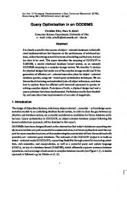
Figure 9: Results of Query 1 We compare the three plans for varying sizes of the argument relation. For all queries, the optimizer selects the first plan. The optimizer generated 12 equivalence classes with 29 class elements. The running times of all plans are shown in Figure 9, where it can be seen that the first two significantly outperform the third. This is because temporal aggregation in the DBMS is very slow. While not reported here, experiments with similar queries, where the the grouping attribute(s) and relation size are also varied, show similar results. This experiment shows that processing in the middleware can be up to ten times faster, if a query involves temporal aggregation. Temporal aggregation in the DBMS can compete with temporal aggregation in the middleware only when a very small number of records (a few hundreds) have to be aggregated (see Query 2). Query 2 “Produce a time-varying relation that provides, for each k`lDm�n�opn�l�q tuple with pay rate greater than $10, the count of employees that were assigned to the position. Consider the time period between January 1, 1983 and January 1, 1984 and sort the result by position number.” This query corresponds to the query presented in Section 2.2, but we introduce the time period and the $10 pay rate condition. Six plans were used, four of which are given in Figure 10. The first plan performs temporal aggregation in the middleware and the rest in DBMS. The next three plans also assign temporal join to the middleware (Plan 2); temporal join and sorting to the middleware (Plan 3); and temporal join, sorting, and selection to the middleware (Plan 4). The fifth plan (not shown) is the same as the first, but no selection is performed on the argument to the temporal aggregation (this selection is not needed for correctness, but it reduces the argument size). The sixth plan (not shown) performs everything in the DBMS.
16
�Wf �� g Query: vw!"-Owy� .t�|O}�x�~ , .�7Ux�~ , ��� !-y-Ovwy ( .y� , .y� ) OvKy� , "-!Ovwy yO
yO
Ov-yO
, Ou�O{-y oft�|O}�x�~ � � � u �F�y �Ot� , t�uwv ( xz.y�x�ui, {�. ) ���O � � t�|O}�x�~ t�|O}�x�~�-{w~ tO � ��O�$ [� -{w~� ..y� $ =.yO
. -{w~� .yO
%$ ..y� -{w3 ~ .y� $ ’1984-01-01’ -{w3 ~ .yO
%$ ’1983-01-01’ y� $ Cond: yO
%$ u � ~O � � � t�|O}�x�~ . p Wf �� g ��� �]� g
/j ]g
y� $ yO
%$
-{w~
t�|O}�x�~ Ou�O{-y (t�|O}�x�~
GroupBy: Aggregate:
�����]�
’1984-01-01’ ’1983-01-01’
GroupBy: Aggregate:
’1984-01-01’ ’1983-01-01’
g� � �� � ����f
t�|O}�x�~ Ou�O{-y (t�|O}�x�~
y��Ot TableName: Cond:
�
)
Dj]g
Attrs:
Join On:
t�|O}�x�~ , �7Ux�~ , y� yO
, Ou�O{-y oft�|O}�x�~ t�|O}�x�~ = t�|O}�x�~
�Wf ��
Query: vw!"-OwyFt�|O}�x�~ , �7Ux�~ , y� , yO
� � u�( � t�uwv xzy�x�ui{ ��O � � �y� $ -{w~(yO
%$ ’1984-01-01’ -{w~�tO � �’1983-01-01’ O� $ u � ~O � � Ft�|O}�x�~ 10
p f ��
-{w~
Query: vw!"-Owy(t�|O}�x�~ , y� , yO
� � u�( � t�uwv xzy�x�ui{ ��O � � Fy� $ u � ~O � � (t�|O’1984-01-01’ }�x�~ , y�
-{w~(yO
%$
’1983-01-01’
)
Plan 2
�Wf �� g Query: vw!"-Owy�t�|O}�x�~ , y� , yO
� � � u �Ft�uwv xzy�x�ui{ ���O � �y� $ -{w~(yO
%$ u � ~O � � Ft�|O’1984-01-01’ }�x�~ , y�
� ’1983-01-01’
g� � �� � ����f
Plan 1
Attrs:
� t�|O}�x�~ , � 7Ux�~ , Ou�O{-y of�t |O}�x�~ , y� , yO
j � ��
Join On:
Cond: y� $
yO
%$
t�|O}�x�~ = t�|O}�x�~
Dj g t�|O}�x�~ Ou�O{-y (t�|O}�x�~ )
GroupBy: Aggregate:
t�|O}�x�~ , y�
F p f �� g
’1984-01-01’ ’1983-01-01’
-{�� w~ ���]�
GroupBy: Aggregate:
�]
t�|O}�x�~ OrderBy:
’1983-01-01’
y� $ yO
%$
Dj]g t�|O}�x�~ Ou�O{-y (t�|O}�x�~ )
� p ��f
-{��w~���]� g ’1984-01-01’
OrderBy:
Cond:
�Wf �� g , �7Ux�~ , y� yO
� � � u �(t�uwv xzy�, x�ui{ ���O � Fy� $ -{w~(yO
$ ’1984-01-01’ -{w~�tO � �’1983-01-01’ �O $ 10
OrderBy:
Cond:
Query: vw!"-Owy(t�|O}�x�~
y� $ -{w~ yO
%$
t�|O}�x�~ , y� �] �����]� g
’1984-01-01’
’1983-01-01’
p f �� g
Query: vw!"-Owy(t�|O}�x�~ , y� , yO
� � u�( � t�uwv xzy�x�ui{
Query: vw!"-OwyFt�|O}�x�~ , y� , yO
� � u�F � t�uwv xzy�x�ui{ ��O � � Fy� $ -{w~(yO
%$ ’1983-01-01’ ’1984-01-01’
Plan 4
Plan 3
Figure 10: Plans for Query 2
17
Attrs:
t�|O}�x�~ , �7Ux�~ , y� yO
, Ou�O{-y oft�|O}�x�~
Join On:
F]
t�|O}�x�~ = t�|O}�x�~
OrderBy:
t�|O}�x�~
��� �]� g Cond: y� $ ’1984-01-01’ -{w~ yO
%$ ’1983-01-01’
�Wf �� Query: vw!"-Owy�t�|O}�x�~ , �7Ux�~ , y� , yO
� � �u �Ft�uwv xzy�x�ui{ ���O � �tO � � �O $ 10
120
300 Plan 1 Plan 2 Plan 3 Plan 4 Plan 5 Plan 6
100
250
200 Time, sec
Time, sec
80
60
150
40
100
20
50
1984
Plan 1 Plan 2 Plan 3 Plan 4 Plan 5 Plan 6
1985
1986
1987
1988
1989
1990
1991
Selection time-period end
1992
1993
1994
1995
1996
1997
1998
Selection time-period end
(a)
(b)
Figure 11: Results of Query 2 when the Selection Time-Period End Value was 1990 or Smaller (a) and 1991 or Bigger (b) We ran all six plans a number of times, each time increasing the end time of the time period given in the query by one year, thus relaxing the predicate. Since most of the k�lDm�n�onl�q data is concentrated after 1992, the running times are similar for the queries with the time period ending before 1992 (see Figure 11), but they increase rapidly after that time (see Figure 11(b)). In Figure 11(a), we also observe that Plans 4 and 5 perform poorly; this is because of the high cost of the p Wf �� operation, which takes the whole base relation as its argument (without applying selection first). Plan 6, which performs temporal aggregation in the DBMS, is competitive because the selection predicates are very selective. For larger time periods (Figure 11(b)), the performances of the plans vary more. Plans 4 and 5 are slow due to the expensive p f �� j operations, and Plan 6 also deteriorates rapidly when the argument to the temporal aggregation increases. Plan 1 deteriorates faster than Plans 2 and 3 because it includes the p Wf �� algorithm, which becomes significantly slower when its argument’s size increases (due to the increase of the selection time period). We optimized this query running the middleware optimizer with and without histograms on the time attributes. When used without histograms, the optimizer returned the second plan for the six queries with the time-period end varying from January 1, 1984 to January 1, 1989, and the first plan for all other queries. When used with histograms, the optimizer always returned the second plan (which is better than the first plan, as is clear from Figure 11(b)), because it could more accurately estimate the result size of the temporal selection. The optimizer generated 142 classes with 452 elements in total. This query shows that temporal join can be as much as two times faster in the middleware if at least one of its arguments resides there (as does, in this case, the result of temporal aggregation). Query 4 shows that the same holds for regular join. In addition, this experiment confirms that the cost-based selectivity estimation helps the middleware optimizer return better plans. Query 3 “For each position in k`lDm�n on�l�q starting before January 1, 1990, show all pairs of employees that occupied that position during the same time. Sort the result by the position number.” This query is a temporal self-join. We tested two plans: the first performs everything in the DBMS, while the second performs temporal join in the middleware. Figure 12 shows two possible plans: the first performs everything in the DBMS, while the second performs temporal join in the middleware. In the experiment, we have varied the condition constraining the time-period start. The running times are shown in Figure 13. When the maximum allowed time for the time-period start increases, Plan 2 performs better than Plan 1 because the result is bigger than the arguments, leading to high costs of sorting within the DBMS and transfer of the result in Plan 1. The difference in performance becomes obvious when the maximum time-period start reaches year 1996, since about 65% of the k`l/m�n�on�lq tuples have time-periods starting at 1995 or later. 18
� t�|O}�x�~ �7Ux�~ �7Ux�~ �Wf �� g j� � �� Attrs: .tO � ��O, . tO � , ��O. �7| , �� } . , . Query: �7| } y�, .yO
vw!"-Owy� .t�|O}�x�~ , .�7Ux�~ , .�7Ux�~ , .Ot � ��O , .tO � ��O , . �� , , �7| �� } �7| �� } ��� !-y-Ovwy � y
y� Ov y� , ( . , . ) "-.!Ovwy ( ,.yO
. ,
.yO
) ,Ov yO
p���f Join On: t�|O}�x�~ = t�|O}�x�~ � � � u ��t�uwv xzy�x�ui{ , t�uwv xzy�x�ui{� ���O � � t�|O}�x�~ t�|O}�x�~ -{w~� ..y� $ =.yO
. -{w~� .yO
$ .y� �Wf �� g p f ��� ] -{w~� .y� $ ’1990-01-01’ -{w3 ~ .y� $ ’1990-01-01’ Query: Query: � w v ! " O w � y � 7 U � x ~ � t O | � } � x ~ O t ��O wv !"-Owy��7Ux�~ , t�|O}�x�~ , tO � ��O , u � ~O � � � .t�|O}�x�~ , �7| �� } , y� yO
, �7| �� } y� yO
, , , � � �u �(t�uwv xzy�x�ui{ � � u��(t�uwv xzy�x�ui,{ ���O � �y� $ ���O � �y� $ u � ~O � � Ft�|O’1990-01-01’ }�x�~ u � ~O � � Ft�|O’1990-01-01’ }�x�~ Plan 1
,
Plan 2 Figure 12: Plans for Query 3
The middleware optimizer returned Plan 1 for the first six queries and Plan 2 for the last three. The errors for the middle three queries—where Plan 2 is already better than Plan 1—occur because the selectivity estimation for join and temporal join assumes uniform distribution of the join-attribute values (k�`Pn� ), which is not the case for the data used. The optimizer generated 104 equivalence classes with 301 element. 450 Plan 1 Plan 2
400 350
Time, sec
300 250 200 150 100 50
1990
1991
1992
1993
1994
1995
1996
1997
1998
Selection time-period start maximum value
Figure 13: Results of Query 3 This query illustrates that allocating processing (in this case, of temporal join) to the middleware can be advantageous if the result size is bigger than the argument sizes. It also demonstrates that the cost-based optimization leads to selecting a better plan for the last three queries. Query 4 “For each employee, compute the number of positions that he or she occupied over time between January 01, 1996 and January 01, 1997. Sort the result by the employee ID.” This query involves temporal aggregation on �� ���n� and a regular join of � Pk ��l������ and k`lDm�n�opn�l�q . Figure 14 shows the first two plans used; the three other plans used may be easily understood in terms of these. The first plan performs temporal aggregation in the middleware and the rest in the DBMS. The second performs both temporal aggregation and join in the middleware, and the third plan performs temporal aggregation, join, and selection in the middleware. The fourth plan is similar to the first plan, but does not perform the initial selection before temporal aggregation, and the fifth plan performs everything in the DBMS. We ran the plans, varying the size of the k`lDm�n on�l�q relation.
��
19
p Wf �� g Query: ���������� � �� �� �� �� ���� �� �� �� �� ���������� �� �������� � ���������� ������������� ������������� � ��� � ����� . , , , , , ��� , , �� ������� �� � ����� �������� ��� � ����� �#" ��$ ��%�&���� � �� �� � ��� ��! , , , , of' �
(�) %�* ��* ,�-���)��.� %�)�����)
� ��* ��%�+���� ' , ' � �� �� �� �� ��� �� . =� . +.� �� ��� �� . �
�
j� � ��
��
� �� ��
������
� ��
���������� � ��
��������� , , , , ���������� ������� ��� � ������������� � ����� , �#� , , ����� �������� � �� ����� � �������� ��� ������� �#" ��$ ��%�&���� �� �� , , , , of' � � � � ��! ��
� �� ��
� �� Join On: = Attrs:
p f �� g ��� � ]
/j ]g
TableName:
Cond:
��*
p���f '
�#"�/ ’1997-01-01’ ��� � � $10 ’1996-01-01’
Cond:
�� ��� �� GroupBy: ��%�&���� �� ��� �� Aggregate: ( )
�1" / ����� ’1997-01-01’ ��$10 ’1996-01-01’
��
� �� GroupBy: ��%�&�� � ��
� �� Aggregate: ( )
p Wf �� Query: ������ ��� �� ��� ��
��� �]�
p f �� Query: ���������� �� ��� �� �� ���� ��
� �� �� ���������� �� �������� � , , , , ���������� ������� ����� ��� ��������� ������� , �#� , , ����� �� ����� � �� � ��� � �������� ��� ������� � � � ��! , %�)�����) +2�� �� �� �
Dj ] p f ��� ]
Query: ������ ���.�� ��� ��
�#" � � $ , ,
�( ) %�* %�� �� �%�� ' ,�-���) � �1" / �����.��$10 ’1997-01-01’ %�)�����) + �� �� �� �1" , �
�#" ��$ , , ( ) %�* %�� ��� �%�� � ' ,�-���) � �1" / �����2� $10 ’1997-01-01’ %�)�����) +2��
� �� �1" , �
’1996-01-01’
Plan 1
’1996-01-01’
Plan 2 Figure 14: Plans for Query 4
The results in Figure 15(a) show that the first plan outperforms the others. This is because the join is faster in the DBMS and it does not require sorted arguments as the p���f algorithm. In addition, p Wf �� j is not very expensive because the cardinality of its argument is small due to the temporal selection, meanwhile, the extra p Wf �� g ’s in Plans 3 and 4 are rather expensive since they retrieve many tuples from the DBMS that are rejected by the ��� � ]g algorithm. For all queries, the middleware optimizer returned Plan 1. It generated 43 equivalence classes and 85 elements. We also ran the plans varying the time-period start; the results are shown in Figure 15(b). The performance of Plan 1 becomes worse than the performance of Plan 2 because p f �� becomes more expensive. The middleware optimizer still returned Plan 1 for all queries because—as for Query 3—the join-attributes did not follow a uniform distribution, as assumed by join selectivity derivation formula. The experiment shows that, in some cases, the middleware can also be used for processing regular DBMS operations. Query 5 “For each position, list the employee name and address.” This query is a regular join of the k`lDm`n�on�l�q and � Pk �Hl������ relations. We tested three plans: the first plan performs sorting and join in the middleware, the second plan performs a nested-loop join in the DBMS, and the third plan performs a sort-merge join in the DBMS (the DBMS join methods were set explicitly using Oracle hints). We executed the plans while varying the size of the k`lDm`n�on�l�q relation. The results in Figure 16(b) show that Plan 2 yields the best performance while the other two plans are competitive. The middleware optimizer suggested to perform the join in the DBMS (plans 2 and 3; since the optimizer does not consider different DBMS join algorithms, both plans were considered as one). It generated 13 equivalence classes with 30 elements in total. This experiment shows that the DBMS is faster when performing queries involving regular operations. The fact that similar algorithms are competitive in the DBMS and middleware (both plans 1 and 3 include sort-merge joins) indicates that the run-time overhead introduced by TANGO is insignificant.
��
20
200
400 Plan 1 Plan 2 Plan 3 Plan 4 Plan 5
Plan 1 Plan 2 Plan 3 Plan 4 Plan 5
350
150
300
Time, sec
Time, sec
250 100
200 150
50
100 50
8K
17K
27K
36K
46K
55K
64K
74K
84K
1996
Table size, rows
1995
1994
1993
1992
Time period start
(a)
(b) Figure 15: Results of Query 4
5.4 Summary of Performance Study Findings The performance experiments demonstrate that the middleware can be very effective when processing queries involving temporal aggregation. Temporal join is faster in the middleware if at least one its arguments already resides there (Query 2), or if its result size is bigger than its argument sizes (Query 3); other experiments not reported here show that there are cases when temporal join is more efficient in the DBMS. In addition, we showed that the cost-based optimization with its simplified cost formulas is effective in dividing the processing between the middleware and the DBMS. The proposed selectivity estimation techniques for temporal selection was shown to more accurately estimate sizes of intermediate relations, which generally results in better plans being selected. Plans allocating all evaluation for the DBMS (including temporal aggregation) perform well for highly selective queries, but deteriorate rapidly as selection predicates are relaxed (Figure 11(b)). For the tested queries, the middleware optimization overhead was very small. We have not implemented the parser and Translator-To-SQL middleware modules, but we do not expect them to significantly slow down the processing. They will use standard language technology and are independent of the database size. It should be noted, though, that we have not tested queries involving many joins; for such queries, it is likely that join-order heuristics should be introduced instead of the join equivalences used (Section 4.2).
6 Related Work The general notion of software external to the DBMS participating in query processing is classic. Much work has been done on heterogeneous databases [HK89, ERS95, OV99] (also called federated databases [SL90] or multidatabases [PBE95]), in which data resident in multiple, not necessarily consistent databases is combined for presentation to the user [RH98, YM98]. This approach shares much with the notion of temporal middleware: the underlying database cannot be changed, the data models and query languages exposed to the users may differ from those supported by the underlying databases, the exported schema may be different from the local schema(s), and significant query processing occurs outside the underlying DBMS. However, there are also differences. A heterogeneous database by definition involves several underlying databases, whereas the temporal middleware is connected to but one underlying database. Hence, in heterogeneous databases, data integration, both conceptually and operationally, is a prime concern; this is a non-issue for temporal middleware. More recently, there has been a great deal of work in the related area of mediators [GP98, Wie92, Wie95] and, more generally, on integration architectures. Roughly, a mediator offers a consistent data model and accessing mechanism to disparate data sources, many of which may not be traditional databases. As such, the focus is on
21
140 Plan 1 Plan 2 Plan 3
120
Time, sec
100
80
60
40
20
8K
17K
27K
36K
46K
55K
64K
74K
84K
Table size, rows
Figure 16: Results of Query 5 resolving schema discrepancies, semi-structured data access, data fusion, and efficient query evaluation in such a complex environment. Again, there are differences between mediators and temporal middleware; the latter does not address issues of data fusion and schematic discrepancies, or of access to semi-structured data. The two approaches, though, share an emphasis on interposing a layer (also termed a wrapper [RS97]) that changes the data model of the data, or allows new query facilities to access the data. Also shared is an emphasis on domain specialization. While the architecture of a temporal middleware is similar at an abstract level to that of a DBMS, the transformation rules, cost parameters, and internal query evaluation algorithms are very different. Several specific related works utilize an integration architecture. The Garlic system [Car98, Haa97] offers access to a variety of data sources, with very different query capabilities. This mediator employs sophisticated cost-based optimization, based on the Starburst optimizer. Notably, the optimizer attempts to push selections, projections, and joins down to the data sources. To do so, it assumes a fixed schema at each data source. The source wrappers require careful calibration and are closely coupled with their sources. In contrast, our approach assumes a single data source supporting the full features of SQL, including schema definition statements. We do not assume that if an operation can be done in a data source, that is best; rather, we permit some query evaluation in the temporal middleware when it is more efficient to do so. Capabilities-based query rewriting [Li98, PGH97, Yer99] also assumes that the data sources vary widely in their query capabilities. Here, attention focuses on capturing the capability of each source, and on using this information in query rewriting. This approach, unlike that just described, is schema independent. Gravano et al. [Pap95] offer a toolkit that allowed wrappers to be automatically generated from high-level descriptions. This approach assumes a specific schema, as well as a fixed query language. In contrast, our approach does not fix the schema. Similarly, [RS97] are concerned with wrapper implementation over diverse data sources; they also fix the schema, and focus on relational projection, selection, and join. Our approach assumes that the underlying database is capable of most, or all, of the processing (though it may not be appropriate for the data source to actually evaluate the entire temporal query). Other mediator systems, e.g., OLE DB [Bla96] and DISCO [Tom97], are similar in their emphases on data integration and access to weak data sources (those with less powerful query facilities). We view mediator approaches as complementary to the temporal middleware approach introduced here. For integrating across diverse data sources, the mediator approach is appropriate. Given such an architecture, a temporal middleware can then be interposed either between the user and the mediator, or between the wrapper and the underlying database. In this way, coarse-grained query processing decisions can be made via the cost-based optimization discussed in Sections 3–4, with more conventional cost-based (and perhaps capabilities-based) optimization making more fine-grained decisions.
22
Several papers discuss layered architectures for a temporal DBMS, e.g., [TJS97], and several prototype temporal DBMSs have been implemented, e.g., [Tiger]. That work is mainly based on a pure translation of temporal query language statements to SQL and does not provide systematic solutions on how to divide the processing of temporal query language statements between the stratum and the underlying DBMS. Vassilakis et al. [VLG98] discussed techniques for adding transaction and concurrency control support to a layered temporal DBMS; their proposed temporal layer always sends regular operators to the DBMS processing and is able to evaluate temporal operators at the end of a query, if needed. Our proposed optimization and processing framework is more flexible. In this paper, we extend our previous foundation for temporal query optimization [SJS00], which included a temporal algebra that captured duplicates and order, defined temporal operations, and offered a comprehensive set of transformation rules. However, that foundation did not cover optimization heuristics, the implementation of temporal operations, or their cost formulas, which are foci of the present paper. Other work on temporal query optimization [GS90, LM93] primarily considers the processing of joins and semijoins. Perhaps most prominently, Gunadhi and Segev [GS90] define several kinds of temporal joins and discuss their optimization. They do not delve into the general query optimization considered here. Vassilakis [Vas00] presents an optimization scheme for sequences of coalescing and temporal selection; when introducing coalescing to our framework, this scheme can be adopted in the form of transformation rules. Related work in selectivity estimation for temporal operators includes [GS90, Seg93, SS00]; we use some of their techniques for estimating the selectivity of temporal predicates (when histograms are not available), and we also show how selectivity can be estimated by using solely statistics available from conventional DBMSs. Several papers have considered cost estimation in heterogeneous systems. Du et al. [DKS92] propose a cost model with different cost formulas for different selection and join methods. Cost factors used in the formulas are deduced in a calibration phase, when a number of sample queries are run on the DBMS. We use a similar approach (recall Section 5.2), but we assume that we do not know the specific algorithms used by the DBMS. Adali et al. [Ada96] argue that predetermined cost models are sometimes unavailable and statistics may not be easily accessible (particularly from non-relational DBMSs); for this scenario, they suggest to estimate the cost of executing a query by using cached statistics of past queries. Because statistics are easily available in our setting, we do not exploit this type of technique. TANGO is implemented using the Volcano extensible query optimizer [GM93] and the XXL library of query processing algorithms [BDS00]. Volcano was significantly extended to include new operators, algorithms, and transformation rules, as well as different types of equivalences (Section 4). Available XXL algorithms for regular operators, as well as our own algorithms for temporal operators, were used in TANGO’s Execution Engine.
7 Conclusions This paper offers a temporal middleware approach to building temporal query language support on top of conventional DBMSs. Unlike previous approaches, this middleware performs some query optimization, thus dividing the query processing between itself and the DBMS, and then coordinates and takes part in the query evaluation. Performance experiments show that performing some query processing in the middleware in some cases improves query performance up to an order of magnitude over performing it all in the DBMS. This is because complex operations, such as temporal aggregation, which DBMSs have difficulty in processing efficiently, have efficient implementations in the middleware. The paper’s contributions are several. It proposes an architecture for a temporal middleware with query optimization and processing capabilities. The middleware query optimization and processing explicitly and consistently address duplicates and order. Heuristics, cost formulas, and selectivity estimation techniques for temporal operators (using available DBMS statistics) are provided. The temporal middleware architecture is validated by an implementation that extends the Volcano optimizer and the XXL query processing system. Performance experiments validate the utility of the shared processing of queries, as well as of the cost-based optimization. The result is a middleware-based system, TANGO, which captures the functionality of previously proposed temporal stratum approaches, and which is more flexible. The proposed transformation rules and selectivity estimation techniques may also be used in an integrated DBMS, e.g., when adding temporal functionality to object-relational DBMSs via user-defined functions. For this to work, the user-defined functions must manipulate relations and must be able to specify the cost functions and transformation rules relevant to them to the optimizer.
23
Several directions for future work exist. The current middleware algorithms should be enhanced to support very large relations. In addition, new operators may be added to TANGO. To add an operator, one needs to specify relevant transformation rules, formulas for derivation of statistics, and algorithm(s) implementing the operator. If the operator is to be implemented in the middleware, its algorithm has to be added to the Execution Engine. DBMS query processing statistics, such as the running times of query parts, may be used to update the cost factors used in the middleware’s cost formulas. It is an interesting challenge to be able to divide the running time between the p f �� j algorithm and, possibly, several DBMS algorithms. A number of other refinements are also possible. For example, if a query is to access the same DBMS relation twice (even if the projected � operation. attributes are different), it would be beneficial to issue only one
Acknowledgments This research was supported in part by the Danish Technical Research Council through grant 9700780, by the U.S. National Science Foundation through grant IIS-9817798, and by a grant from the Nykredit Corporation.
References [Ada96] S. Adali, K. S. Candan, Y. Papakonstantinou, and V. S. Subrahmanian. Query Caching and Optimization in Distributed Mediator Systems. In Proceedings of ACM SIGMOD, Montreal, Canada, pp. 137–148 (1996) [BDS00] J. Van der Bercken, J. P. Dittrich, and B. Seeger. javax.XXL: A Prototype for a Library of Query Processing Algorithms. In Proceedings of ACM SIGMOD, Dallas, TX, p. 588 (2000). [Bla96] J. Blakeley. Data Access for the Masses Through OLE DB. In Proceedings of ACM SIGMOD, Montreal, Canada, pp. 161–172 (1996). [Boe95] M. H. B¨ohlen. Temporal Database System Implementations. ACM SIGMOD Record, 24(4): 53–60 (1995). [Car98] M. J. Carey, L. M. Haas, J. Kleewein, and B. Reinwald. Data Access Interoperability in the IBM Database Family. Data Engineering Bulletin, 21(3): 4–11 (1998). [DKS92] W. Du, R. Krishnamurthy, and M.-C. Shan. Query Optimization in a Heterogeneous DBMS. In Proceedings of VLDB, Vancouver, Canada, pp. 277–291 (1992). [EJS98] O. Etzion, S. Jajodia, and S. Sripada (eds.). Temporal Databases: Research and Practice. LNCS 1399. Springer-Verlag (1998). [EN00] R. Elmasri and S. B. Navathe. Fundamentals of Database Systems. Third Edition. Addison-Wesley (2000). [ERS95] A. Elmagarmid, M. Rusinkiewicz, and A. Sheth. Heterogeneous Distributed Databases. Morgan Kaufmann (1995). [GM93] G. Graefe and W. J. McKenna. The Volcano Optimizer Generator: Extensibility and Efficient Search. In Proceedings of IEEE ICDE, Vienna, Austria, pp. 209–218 (1993). [GP98] L. Gravano and Y. Papakonstantinou. Mediating and Metasearching on the Internet. Data Engineering Bulletin 21(2): 28–36 (1998). [GS90] H. Gunadhi and A. Segev. A Framework for Query Optimization in Temporal Databases. In Proceedings of SSDBM, Charlotte, NC, pp. 131–147 (1990). [Haa97] L. M. Haas, D. Kossmann, E. L. Wimmers, and J. Yang. Optimizing Queries Across Diverse Data Sources. In Proceedings of VLDB, Athens, Greece, pp. 276–285 (1997). [HK89] D. Hsiao and M. Kamel. Heterogeneous Databases: Proliferation, Issues, and Solutions. IEEE TKDE, 1: 45–62 (1989). 24
[Inm96] W. H. Inmon. Building the Data Warehouse. Second Edition. John Wiley and Sons (1996). [Ioa96] Y. Ioannidis. Query Optimization. ACM Computing Surveys, 28(1): 121–123 (1996). [Jar84] M. Jarke and J. Koch. Query Optimization in Database Systems. ACM Computing Surveys, 16(2): 111– 152 (1984). [JS99] C. S. Jensen and R. T. Snodgrass. Temporal Data Management. IEEE Transactions on Knowledge and Data Engineering, 11(1):36–45, 1999. [KS95] N. Kline and R. T. Snodgrass. Computing Temporal Aggregates. In Proceedings of IEEE ICDE, Taipei, Taiwan, pp. 222–231 (1995). [Li98] C. Li, R. Yerneni, V. Vassalos, H. Garcia-Molina, Y. Papakonstantinou, J. D. Ullman, and M. Valiveti. Capability Based Mediation in TSIMMIS. In Proceedings of ACM SIGMOD, Seattle, WA, pp. 564–566 (1998). [LM93] T. Y. C. Leung and R. R. Muntz. Stream Processing: Temporal Query Processing and Optimization. In Temporal Databases: Theory, Design, and Implementation, A. U. Tansel et al. (eds.), Benjamin/Cummings, pp. 329–355 (1993). [OV99] T. M. Ozsu and P. Valduriez. Principles of Distributed Database Systems. Second Edition. Prentice Hall (1999). [Pap95] Y. Papakonstantinou, A. Gupta, H. Garcia-Molina, and J. Ullman. A Query Translation Scheme for Rapid Implementation of Wrappers. In Proceeding of DOOD, Singapore, pp. 161–186 (1995). [PBE95] E. Pitoura, O. Bukhres, and A. Elmagarmid. Object Orientation in Multidatabase Systems. ACM Computing Surveys, 27(2): 141–195 (1995). [PGH97] Y. Papakonstantinou, A. Gupta, and L. Haas. Capabilities-Based Query Rewriting in Mediator Systems. Distributed and Parallel Databases, 6(1): 73–110, (1998). [RH98] F. de Ferreira Rezende and K. Hergula. The Heterogeneity Problem and Middleware Technology: Experiences with and Performance of Database Gateways. In Proceedings of VLDB, New York, NY, pp. 146–157 (1998). [RS97] M. T. Roth and P. M. Schwarz. Don’t Scrap it, Wrap It! A Wrapper Architecture for Legacy Data Sources. In Proceedings of VLDB, Athens, Greece, pp. 266–275 (1997). [Seg93] A. Segev, G. Himawan, R. Chandra, and J. Shanthikumar. Selectivity Estimation of Temporal Data Manipulations. Information Sciences, 74(1-2): 111–149 (1993). [SJS00] G. Slivinskas, C. S. Jensen, and R. T. Snodgrass. Query Plans for Conventional and Temporal Queries Involving Duplicates and Ordering. In Proceedings of IEEE ICDE, San Diego, CA, pp. 547–558 (2000). [SL90] A. Sheth and L. Larson. Federated Database Systems for Managing Distributed, Heterogeneous, and Autonomous Databases. ACM Computing Surveys, 22(3): 183–236 (1990). [Sno99] R. T. Snodgrass. Developing Time-Oriented Database Applications in SQL. Morgan Kaufmann (1999). [SS00] I. Sitzmann and P. J. Stuckey. Improving Temporal Joins Using Histograms. In Proceedings of DEXA, London/Greenwich, UK, pp. 488–498 (2000). [SSJ94] M. D. Soo, R. T. Snodgrass, and C. S. Jensen. Efficient Evaluation of the Valid-Time Natural Join. In Proceedings of IEEE ICDE, Houston, TX, pp. 282–292 (1994).
�
[Tiger] M. H. B¨ohlen. The Tiger Temporal Database System. URL: www.cs.auc.dk/˜tigeradm/ (current as of February 23, 2001).
[TJS97] K. Torp, C. S. Jensen, and R. T. Snodgrass. Stratum Approaches to Temporal DBMS Implementation. In Proceedings of IDEAS, Cardiff, Wales, pp. 4–13 (1998). 25
[TJS00] K. Torp, C. S. Jensen, and R. T. Snodgrass. Effective Timestamping in Databases. The VLDB Journal, 8(3-4): 267–288 (2000). [Tom97] A. Tomasic, R. Amouroux, P. Bonnet, O. Kapitskaia, H. Naacke, and L. Raschid. The Distributed Information Search Component (Disco) and the World Wide Web. In Proceedings of SIGMOD, Tucson, AZ, pp. 546–548 (1997). [UIS] J. A. G. Gendrano, R. Shah, R. T. Snodgrass, and J. Yang. University Information System (UIS) Dataset. T IME C ENTER CD-1, September, 1998. [Vas00] C. Vassilakis. An Optimisation Scheme for Coalesce/Valid Time Selection Operator Sequences. SIGMOD Record, 29(1): 38–43 (2000). [VLG98] C. Vassilakis, N. A. Lorentzos, and P. Georgiadis. Implementation of Transaction and Concurrency Control Support in a Temporal DBMS. Information Systems, 23(5): 335–350 (1998). [Wie92] G. Wiederhold. Mediators in the Architecture of Future Information Systems. IEEE Computer, 25(3): 38–49 (1992). [Wie95] G. Wiederhold. Mediation in Information Systems. ACM Computing Surveys, 27(2): 265–267 (1995). [Yer99] R. Yerneni, C. Li, H. Garcia-Molina, and J. D. Ullman. Computing Capabilities of Mediators. In Proceedings of ACM SIGMOD, Philadelphia, PA, pp. 443–454 (1999). [YM98] C. Yu and W. Meng. Principles of Database Query Processing for Advanced Applications. Morgan Kaufmann (1998). [YYW00] J. Yang, H. C. Ying, and J. Widom. TIP: A Temporal Extension to Informix. In Proceedings of ACM SIGMOD, Dallas, TX, p. 596 (2000).
26