Adaptations of k-Shortest Path Algorithms for ... - UNIV-TLSE3

Adaptations of k-Shortest Path Algorithms for Transportation Networks Gr´egoire Scano, Marie-Jos´e Huguet, Sandra Ulrich Ngueveu

To cite this version: Gr´egoire Scano, Marie-Jos´e Huguet, Sandra Ulrich Ngueveu. Adaptations of k-Shortest Path Algorithms for Transportation Networks. International Conference on Industrial Engineering and Systems Management, Oct 2015, Seville, Spain. 2015.

HAL Id: hal-01207475 https://hal.archives-ouvertes.fr/hal-01207475 Submitted on 30 Sep 2015

HAL is a multi-disciplinary open access archive for the deposit and dissemination of scientific research documents, whether they are published or not. The documents may come from teaching and research institutions in France or abroad, or from public or private research centers.

L’archive ouverte pluridisciplinaire HAL, est destin´ee au d´epˆot et `a la diffusion de documents scientifiques de niveau recherche, publi´es ou non, ´emanant des ´etablissements d’enseignement et de recherche fran¸cais ou ´etrangers, des laboratoires publics ou priv´es.

Adaptations of k -Shortest Path Algorithms for Transportation Networks c I4 e2 2015 (presented at the 6th IESM Conference, October 2015, Seville, Spain)

Gr´egoire Scano∗

† §,

Marie-Jos´e Huguet∗

†

and Sandra Ulrich Ngueveu∗

‡

∗ CNRS,

LAAS, 7 avenue du colonel Roche, F-31400 Toulouse, France Toulouse, INSA, LAAS, F-31400 Toulouse, France ‡ Univ Toulouse, ENSEEIHT, LAAS, F-31400 Toulouse, France § MobiGIS, ZAC Grenade Sud, Rue de l’Autan, F-31330 Grenade, France † Univ

Email: {gscano, huguet, sungueve}@laas.fr Abstract—The computation of the k-shortest paths, should they be elementary or not, has been extensively investigated in the literature, yielding to extremely performant algorithms. For elementary paths, the best known algorithm to this day is the algorithm of Yen enhanced by the extension of Lawler, while for the search of non-elementary paths, the algorithm with the best complexity is due to Eppstein but is outperformed in practice by the Recursive Enumeration Algorithm. In the context of transportation networks, graphs are time dependent, meaning that the cost of an edge depends on the time at which it is crossed. If for each edge one cannot arrive later if he departs earlier, the network is said to respect the FIFO property. Under this hypothesis, the usual Dijkstra shortest path algorithm is still polynomial. Additionally, since each edge is associated to a transportation type, one may want to restrict a path to be in a regular language. To find a shortest path under this constraint a polynomial algorithm, called DRegLC, works on the product of the network and the graph representing an automaton accepting the regular language. In this paper, some k-shortest paths algorithms are adapted to be used on such transportation networks with a regular language constraint. Also, the computation of the k-shortest elementary paths is considered using k-shortest non elementary paths algorithms, deleting loops while searching if possible. To address this approach, a new algorithm is presented to speedup the search of elementary paths while scanning as few paths containing loops as possible.

I.

I NTRODUCTION AND P ROBLEM STATEMENT

Computing efficiently the shortest path in the context of transportation networks, including multimodality and timedependency, has been the subject of intensive research in the last ten years. However, users of transportation networks can be interested not only in the shortest path between the origin and the destination of their journey but also in a set of viable paths. Moreover, public transport authorities and city planners may be interested by information about the number of paths and associated durations or costs, connecting two points or areas, in order to improve their transport offer. This can be done by considering k-shortest paths methods producing a set of paths ordered by their costs. The kshortest paths problem is a well-known problem and it was studied from two points of view depending on the application: producing a set of paths without cycles or producing paths with no restrictions on cycles. The former set is a subset of

the later. In the literature, paths with no restriction on cycles are simply denoted paths with cycles. The k-shortest paths algorithms producing paths with cycles have lower worst-case complexities than algorithms producing only cycle-free paths. In the multimodal transportation context, the aim is to produce k-shortest paths from a given origin to a given destination without any cycle and going through the public transportation network and the pedestrian network. Obviously, in transportation applications, users are not interested in paths having cycles. However, due to the difference in algorithms complexity when considering paths with or without cycles and due to the specific topology of transportation networks (with bus lines for instance), both approaches have merits. Of course, as we do not consider a path with cycles as an admissible solution for users, those paths have to be removed from the set of paths generated. Therefore, when considering k-shortest paths with cycles, one would have to produce a high number of paths to obtain the expected number of paths without cycles. Let G(V, A) be a directed graph, where V is a set of n nodes and A a set of m arcs and let us consider a static positive cost ci,j on each arc (i, j). A path is defined by a sequence of consecutive arcs (or by the sequence of their corresponding nodes). On such graphs, given an origin node o, and a destination node d, solving the Shortest Path problem consists in finding the path from o to d having the minimal cost and solving the k-Shortest Paths problem consists in finding a set of k paths from o to d having minimal costs if possible: no path outside of this set has a cost lower than any path of the set. The k-Shortest Paths problem on static weighted graphs was already studied in the literature, but the specific case of transportation graphs was not studied. A Transportation Network is not modeled using static weighted graphs, but it is based on labeled directed graphs GL (V, A, Σ) consisting of a set of n nodes v ∈ V, a set of m labeled arcs (i, j, l) ∈ A ⊆ V × V × Σ, and a set of p labels l ∈ Σ. Each triplet (i, j, l) represents an arc from node i to node j having label l. The labels on arcs represent transportation modes, such as foot, car, bus, metro, etc. Moreover a positive cost corresponding to the travel time is associated to each arc. Costs may be time-dependent (considering for example timetables or frequency of public transportation lines) and ci,j,l (t) gives the cost of an arc (i, j, l) when arriving at i at time t. The integration of multimodality through labels or timedependent costs increases the complexity of Shortest Paths

algorithms because it restricts the application of some efficient techniques such as bidirectional ones. To the best of our knowledge, there is no dedicated algorithm taking into account both multimodality and time-dependency, for solving the k-Shortest Paths Problem in the context of transportation networks. The rest of the paper is organized as follows. In Section II, we recall the k-Shortest Paths problems previously studied for static weighted directed graphs and the associated algorithms. Then, in Section III, we introduce three algorithms designed for solving the k-Shortest Paths problem in Transportation Networks. Last, in Section IV, we evaluate our algorithms on a real transportation network, before concluding in Section V. II.

R ELATED W ORK

In a static weighted graph G(V, A), given an origin node o and a destination node d, the Shortest Path problem (SP) from o to d is solved in polynomial time with the well-known D I S J K S T R A algorithm. In this algorithm, a label is associated to each node, each label containing the current shortest path from the origin to the corresponding node. Two main speed-up techniques were introduced to improve the efficiency of this algorithm: A* and bidirectionnal search. Hart [1] proposed the A∗ algorithm, where a D I S J K S T R A algorithm is guided towards the destination informed by an estimate cost between the current node and the destination d. Obtaining the optimal solution at the end of such algorithm is guaranteed if the estimation is a lower bound of the exact cost. Its complexity is the same as of D I S J K S T R A if the triangle equality is valid on any node with respect to this estimate. A bidirectional algorithm, explained by Nicholson, [2] is not more informed than D I S J K S T R A but two searches are conducted from origin to destination (forward search) and conversely on the reverse graph (backward search). When a connection is found between the forward and the backward searches, a feasible solution is obtained. Such solution is optimal if and only if its cost is less or equal to the sum of the minimum forward and backward costs of the partial paths that remain unexplored. Some extensions of the SP problem were proposed to deal with the time-dependency of travel times. It has been shown in [3] that the resolution of the SP problem with such a cost is polynomial iff the arcs in the graph respect the FIFO property (any path starting with a greater cost from a given node will have a greater final cost than any other path starting with a lower cost from the same departure node and arriving at the same final node). However, many efficient techniques based on bidirectional search cannot be easily extended in the time-dependent case as the exact starting time is only given at the origin. In Transportation Networks, the sequence of modes corresponding to a path can be restricted to a language to take into account user or mode constraints. The regular language constrained shortest path problem can be solved in polynomial time [4] using the DRegLC algorithm presented in [5] that is an extension of the D I S J K S T R A algorithm on the product graph of G (a directed weighted graph) and the automaton accepting the given regular language L. Regarding bidirectional search and assuming that the automaton is deterministic, bidirectional methods despite correctness, may be exponentially complex if the reverse

automaton is non deterministic since crossing backward an arc from a given state may result into several non dominated states. A path in a graph is a sequence of consecutive arcs and will be denoted π, the associated sequence of nodes will be denoted by π. A path π is said to be simple iff it contains at most once any arc. A path π is an elementary path iff it is simple and has no cycle, i.e., no node occurs more than once. The ith node (resp. arc) in π (resp. π) is denoted π[i] (resp. π[i]) and π(i, j) (resp. π(i, j)) denotes the path from node i to node j. The k-shortest paths (k-SP) problem consists in computing a given number of non decreasing cost paths between two nodes. Depending on the type of required paths (elementary or unrestricted), different types of algorithms exist in the literature. Yen’s algorithm [6] computes the k elementary shortest paths. It uses a shortest path algorithm as a subroutine and successively calls it from different origins after discarding from the graph previously used edges. The complexity of the algorithm is O(k.n.SP (n, m)) where SP (n, m) is the complexity of the shortest path algorithm being used. Computing k paths without any restriction on cycles, also known as paths with cycles, is easier than computing elementary paths since there is no need to track and prevent the occurrence of loops within the paths. The algorithm of Eppstein [7] runs with an excellent complexity of O(m + n.log(n) + k.log(k)). Unfortunately, Eppstein’s algorithm cannot be extended efficiently to time-dependent graphs since it uses as a first step the computation of a backward shortest path tree, which is not possible since the costs of arcs depend on the starting time, and therefore can only be known during a forward exploration. It can be observed that to compute the k th path, only nodes in the k th − 1 path have to be explored. The REA algorithm [8] uses this fact to compute paths with cycles with a higher complexity of O(m + k.n.log(n)), but the running time in practice is better than that of Eppstein’s. In addition, this idea can be applied to make a lazy version of the former algorithm [9] by delaying the construction of some parts of the intermediary graph. Such adaptation does not change the worst case complexity. In the context of multimodal and time-dependent graphs (i.e. transportation networks), there is no dedicated k-shortest paths algorithms and there is no comparison of the both types of algorithms (with and without cycles). Due to the specificities of such graphs, we propose to evaluate the efficiency of both approaches (with and without cycles) and to do that we present, in the next Section, two extensions and one new variant of kshortest paths algorithms. III.

P ROPOSED A LGORITHMS

In the following, the computation of the k-shortest paths is always done in the context of a multimodal time-dependent network. Thus, we consider any regular language and the automaton that accepts it to represent mode constraints (if the automaton is non deterministic, we determine it). Our goal is to

determine k-shortest paths without cycles for a given origin o, a given destination d and a given start time t at the origin. We consider the two types of k-SP approaches: with or without cycles. In the case of k-SP with cycles, paths that contain cycles are disregarded after the search and some cycles may also be eliminated during the search. A. Extension for k-shortest paths without cycles In Yen’s algorithm [6], the shortest path is computed first (using D I J K S T R A procedure), then each node of this shortest path is considered to compute another shortest path to the destination. This principle is successively applied on each node of previously obtained paths. When computing k-shortest paths using such method, some nodes and edges need to be removed from the graph (to find different paths) and are ignored by the search by tapping directly into D I J K S T R A internal data structures. The Lawler’s extension [10] prevents from recomputing previously enumerated paths. For time-dependent and multimodal graphs, the extension of Yen’s (or Lawler’s) algorithm is straightforward using the DRegLC algorithm as the sub-procedure instead of the D I J K S T R A algorithm and produces a set of paths without cycle. B. Extension for k-shortest paths with cycles Eppstein’s algorithm solves as a first step the shortest path tree rooted at the destination. It then builds an intermediate tree structure representing every possible deviation along the shortest path tree with respect to arcs in the graph. To allow multiple deviations to happen along a path, leaves are connected to the root. Then, a k shortest path algorithm can be applied on the resulting compacted tree yielding to much better performances in finding the shortest paths since it just combines deviations in every possible way instead of exploring them multiple times on the graph. However, when considering time-dependency, it was already shown that backward search is based on lower bounds and then re-computation, and therefore increases computation times. Moreover, taking into account multimodality may require non-deterministic automaton to represent mode constraints, leading to an additional increase of computation time. Instead of Eppstein’s algorithm, we consider the adaptation of the REA algorithm that also computes k shortest paths with cycles. The REA algorithm, starts with a standard one-to-all shortest path algorithm. Then, it works in a recursive way and starts at the destination node to compute the next shortest path. Each node produces then a set of labels corresponding to paths. This list of labels is initialized when the second shortest path is required by extending the computed paths coming from nodes not in the shortest path to the considered node. It is then extended by recursive computations of shortest paths from nodes on the previous shortest path. The adaptation of this algorithm for taking into account both multimodality and time-dependency is immediate. C. New variant of k-shortest paths algorithm with cycles In addition, we propose another algorithm close to REA but working in an iterative way to compute k shortest paths with cycles between an origin o and a destination d. This

algorithm, denoted as Iterative Enumeration Algorithm or IEA, computes the shortest path from o to all of the other nodes using a D I S J K S T R A -like procedure. The main difference is that several labels can be stored on each node, even if the corresponding node was already visited and therefore marked. Moreover, another mark and an index are directly associated to each label on each node. A label is marked if it has already been selected and propagated. Of course, priority is given to the labels of minimal cost. The index on the label represents an identifier of the label (to re-compute the produced path); indexes are produced in increasing order. For a given node x, one associates a Boolean mark Bx to state whether this node was already visited or not, and a label lx defined by lx = (c, p(r0 ), r, b) where c is the current cost from the origin to x, p the predecessor node, r0 the index of the label on node p, r the index of label on node x and b a Boolean mark to state whether this label was already considered or not. Initially, all nodes are unmarked (not visited), the cost of all labels is set to infinity except for the origin that has a label with cost 0 (and index 1), and all labels are unmarked. The main steps of the IEA algorithm are the following: 1) 2) 3)

4)

select the unmarked node having the unmarked label with the lowest cost, mark this node and this label as visited; add new labels for each successor nodes, even if these nodes are marked, and number the produced labels; when the destination node is selected in step 1 and marked (a label for this node is also marked), store the solution and increase the count on the number of produced paths. Then, unmark all nodes belonging to the shortest path (note that marks remain on labels). restart at step 1 with the new set of unmarked nodes and labels. This set is composed only of nodes belonging to the previously obtained path and of nodes not visited during the previous search.

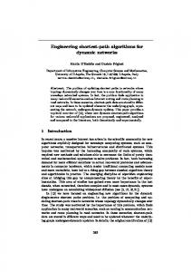
The algorithm stops when the required number of paths is obtained or when there is no remaining unmarked node or when there is no remaining unmarked labels. Note that in this algorithm, we can also suppress cycles going through the origin by do not allow to unmark the origin in step 3 (and do not produce new labels on the origin in step 2). Let us consider the example given in figure 1 with 4 nodes. The origin is x1 and the destination x4 . In this small example, there are 4 different paths without cycle: π 1 = {x1 , x2 , x4 } with cost 4, π 2 = {x1 , x2 , x3 , x4 } with cost c(π 2 ) = 4, π 3 = {x1 , x3 , x2 , x4 } with cost c(π 3 ) = 10 and π 4 = {x1 , x3 , x4 } with cost c(π 4 ) = 11. In the proposed algorithm node x1 received a label lx1 = (0, ∅, 1, f alse) and it is not visited (vx1 = f alse). In table I, we detail the labels produced on each node. At the beginning, the origin x1 is selected, marked as visited, its label is also marked as visited and it is propagated through x2 and x3 (line1). In line 2, the unmarked node x2 has the unmarked label with lowest cost (1), it is marked as visited, its label is also marked and its successors receive new labels (nodes x3 and x4 ). In line 3, node x3 is selected as it is unmarked and has the lowest cost (3) and produce new labels on node x2

x2

2

x1

x4

5

Toy example for the computation of k-shortest paths

TABLE I. step 1 2

L ABELS PRODUCED DURING THE IEA A LGORITHM

x2 (F; {(1, x1 (1), 1, F)}) (T; {(1, x1 (1), 1, T)})

5

(T; {(1, x1 (1), 1, T), (5, x3 (2), 2, F)}) (T; {(1, x1 (1), 1, T), (5, x3 (2), 2, F)}) (T; {(1, x1 (1), 1, T), (5, x3 (2), 2, T) })

6

(T; {(1, x1 (1), 1, T), (5, x3 (2), 2, T) })

3 4

(F; {(1, x1 (1), 1, T), (5, x3 (2), 2, T), (7, x3 (1), 3, F) })

8

K: the counter of found solutions for each node,

•

lc: the length of cut-cycle,

•

S: the solution set.

6

x3 Fig. 1.

• 3

1

x3 (F; {(5, x1 (1), 1, F)}) (F; {(5, x1 (1), 1, F), (3, x2 (1), 2, F)}) (T; {(5, x1 (1), 1, F), (3, x2 (1), 2, T)}) (T; {(5, x1 (1), 1, F), (3, x2 (1), 2, T)}) (T; {(5, x1 (1), 1, F), (3, x2 (1), 2, T), (7, x2 (2), 3, F) }) (T; {(5, x1 (1), 1, F), (3, x2 (1), 2, T), (7, x2 (2), 3, F) }) (T; {(5, x1 (1), 1, T), (3, x2 (1), 2, T), (7, x2 (2), 3, F) })

9

(T; {(1, x1 (1), 1, T), (5, x3 (2), 2, T), (7, x3 (1), 3, T) })

(T; {(5, x1 (1), 1, T), (3, x2 (1), 2, T), (7, x2 (2), 3, F), (9, x2 (3), 4, F) })

10

(T; {(1, x1 (1), 1, T), (5, x3 (2), 2, T), (7, x3 (1), 3, T) })

(T; {(5, x1 (1), 1, T), (3, x2 (1), 2, T), (7, x2 (2), 3, F), (9, x2 (3), 4, F) })

x4 (F, {(4, x2 (1), 1, F)}) (F, {(4, x2 (1), 1, F), (9, x3 (2), 2, F)}) (T, {(4, x2 (1), 1, T), (9, x3 (2), 2, F)}) (F, {(4, x2 (1), 1, T), (9, x3 (2), 2, F), (8, x2 (2), 3, F) }) (T, {(4, x2 (1), 1, T), (9, x3 (2), 2, F), (8, x2 (2), 3, T) }) (F, {(4, x2 (1), 1, T), (9, x3 (2), 2, F), (8, x2 (2), 3, T), (11, x3 (1), 4, F) }) (F, {(4, x2 (1), 1, T), (9, x3 (2), 2, F), (8, x2 (2), 3, T), (11, x3 (1), 4, F), (10, x2 (3), 5, F) }) (T, {(4, x2 (1), 1, T), (9, x3 (2), 2, T), (8, x2 (2), 3, T), (11, x3 (1), 4, F), (10, x2 (3), 5, F) })

and x4 . Then, in line 4, the only unmarked node is x4 , and the algorithm obtains the first path with cost 4, this label is marked on x4 . Nodes belonging to this path (π 1 = {x1 , x2 , x4 }) are unmarked, except the origin. The algorithm re-starts with two unmarked nodes x2 and x4 . The node having the unmarked label with the lowest cost is x2 (cost 5). In line 5, this node and its label are marked and produce new labels on nodes x3 and x4 . Node x3 is marked and cannot be selected. The only unmarked node is x4 with cost 8 (line 6) producing the second path: π 2 = {x1 , x2 , x3 , x2 , x4 } (path with a cycle). Then all nodes except the origin are unmarked and the algorithm re-starts. The node having the lowest cost is x3 that is marked and new labels are produced on x2 and x4 (line 8). In line 9, node x2 is selected (cost 7) and produces new labels on x3 and x4 . Then, in line 9, node x4 has the lowest cost (9) and a new path is obtained: π 3 = {x1 , x2 , x3 , x4 }. The algorithm re-starts again with all nodes set as not-visited. In Algorithm 1, we detail the proposed Iterative Enumeration Algorithm integrating cut-cycles with the following variables : •

L: the set of labels for each node and each index,

•

B: the set of marks for each node,

•

H: the heap of candidate labels,

At the beginning, the heap is initialized with the label of the origin o having a given cost c0 . Then, while the number of solutions k 0 has not been found, the algorithm selects the best available label in H and as it gets extended iff it does not introduce any cycle of length lc. When a path is found, i.e. the node solution is unstacked but with a value of k 0 lower than the given argument, every node in the associated path is made available for the next step. The complexity of this algorithm is the same as of REA, i.e. O(m+k.n.log(n)). The IEA algorithm can be directly adapted for time-dependent and multimodal graphs. Algorithm 1 Iterative Enumeration Algorithm Require: G = (V, E), o, d, k0 , f : E × E → R+ , lc, c0 Ensure: S = {(k∗, c∗)} 1: 2: 3: 4: 5: 6: 7: 8: 9: 10: 11: 12: 13: 14: 15: 16: 17: 18: 19: 20: 21: 22: 23: 24: 25: 26: 27: 28: 29: 30: 31: 32: 33: 34: 35: 36: 37: 38: 39: 40: 41: 42:

. Initialize Lx,0 ← (∞, ∅, 0, f alse), ∀x ∈ V Lo,0 ← (c0 , ∅, 0, f alse) Bx ← lc, ∀x ∈ V H ← Lo,0 Kx ← 0, ∀x ∈ V S←∅ . Select the unmarked label with minimal cost, mark the node and the label while H 6= ∅ ∧ Kd 6= k0 do lx = (c, p(r0 ), r, b) ← minBx 0 (H) H ← H \ {lx } Bx ← Bx − 1 b ← true Kx ← Kx + 1 if x 6= d then . Produce sucessor labels ly for y ∈ {z ∈ V \ {o} | (y, z) ∈ E} do . check cycles (cycle, count) ← (f alse, lc) lz = (−, qz (rz0 ), −, −) ← lx while count 6= 0 do if z = x then (cycle, count) ← (true, 0) end if (count, lz ) ← (count − 1, Lqz ,rz0 ) end while if ¬cycle then ly ← (c + f (x, y), x(r), |Lx | + 1, f alse) H ← H ∪ {ly } end if end for else . unmark the obtained path S ← S ∪ (Kx , c) ly = (−, qy (ry0 ), ry , −) ← lx while y 6= o ∧ ry 6= 1 do By ← By + 1 ly ← Lqy ,ry0 end while end if end while return S

TABLE II.

D. Cutting cycles during the search When using REA or IEA algorithms, one produces (with a low worst-case complexity) k shortest paths with cycles, then due to the application, paths with cycles are disregarded. We consider here, how to adapt these two algorithms to suppress some cycles during the search. 1) Embedding cut cycles in REA algorithm: The REA algorithm produces paths with cycles via the origin and the destination nodes. Considering our application, we propose to modify REA algorithm to forbid cycles going through the origin by not allowing recursive calls on the origin node. However, concerning cycles at the destination, only part of them could be removed by preventing every other node to pull path stubs from the destination when k equals to 2, i.e. at the initialization of paths on a node. Also, for every other path, even if cycles can be detected using local storage, removing a cycle within a recursive call would cause the evaluation to stall on the computation of another path with a different k value, yielding to an impractical approach. 2) Embedding cut cycles in IEA algorithm: In the IEA algorithm, we propose to suppress some cycles during the search by checking whether a successor node is or not in the predecessor list of the node having the label with the minimal cost. The size of the predecessor list directly impacts the size of removed cycles. However, when introducing this cycles removal, the shortest paths may appear in a non-increasing order. For instance, let us consider the example given in figure 2 in which we only consider the direct predecessors of each node when extending a label. The origin is x1 and the destination x2 . In this example, there are 5 different paths without cycle: π 1 = {x1 , x2 } with cost 3, π 2 = {x1 , x3 , x2 } with cost c(π 2 ) = 7, π 3 = {x1 , x4 , x5 , x3 , x2 } with cost c(π 3 ) = 13, π 4 = {x1 , x3 , x5 , x2 } with cost c(π 4 ) = 14 and π 5 = {x1 , x4 , x5 , x2 } with cost c(π 5 ) = 16. x2

3

time 23 849 49 276 76 052 100 371 125 666 248 875

cost 81.403 81.404 81.406 81.407 81.408 81.412

dev c 0.015 0.093 0.155 0.171 0.199 0.301

hops 90.65 91.17 91.63 91.84 91.93 92.88

dev h 4.16 4.44 4.51 4.36 4.47 4.53

max time 50 712 102 012 153 787 205 532 257 166 519 595

iteration, the label {(10, x3 (1), 1)} on x5 is extended to x3 to obtain the label {(12, x5 (2), 2)} and the label {(16, x5 (2), 4)} on x2 , but there is no new label on x4 as it is a predecessor of the considered label. Then, the path having cost 13 is obtained. At the last iteration, the path with cost 16 is produced. With this example, one can see that the paths are not produced in an increasing order of their cost. Then, using cut-cycles in the IEA algorithm leads to a heuristic approach to obtain the k-shortest paths when limiting the number of produced paths. IV.

E XPERIMENTAL R ESULTS

The tests were carried out on an Intel(R) Core(TM) i53337U CPU @ 1.7GHz with 6144 KB cache and 3GB main memory, running Linux 3.2.0.4-amd64. All algorithms were implemented in C++ and compiled with GCC. Regarding the instances, we used as transportation network a multimodal graph modeling the city of Toulouse (France). All transportation data used are freely available data: the road network corresponds to the OpenStreetMap data sets and was provided by GeoFabrik and our public transportation network is based on The General Transit Feed Specification format. Once converted into an edge-labeled multimodal graph, it contains 75 837 nodes, 484 426 road edges and 43 318 public transport edges. All combinations of public transportation modes are authorized, including pedestrian. A generic automaton that allows walk, bus and subway is used and the departure time is set to 9 AM.

1

x1

6 6

x3

7

2

x4 Fig. 2.

k 10 20 30 40 50 100

R ESULTS FOR Y EN ’ EXTENSION

x5

3

Heuristic cycles cut

When computing the first path, the IEA algorithm produces the following labels: {(3, x1 (1), 1)} on x2 , {(6, x1 (1), 1)} on x3 , and {(7, x1 (1), 1)} on x4 . Then the path having cost equals to 3 is obtained on the destination x2 . At the next iteration for the computation of the second path, labels {(6, x1 (1), 1)} on x3 , and {(7, x1 (1), 1)} on x4 are marked and new labels are produced: {(8, x3 (1), 1)} on x5 , {(7, x3 (1), 2)} on x2 and {(10, x3 (1), 1)} on x5 . The path having cost equals to 7 is then obtained on the destination. During the following iteration, the label {(8, x3 (1), 1)} on x5 cannot be extended on x3 as x3 is the predecessor of this label but it is extended on node x2 with label {(14, x5 (1), 3)} and on node x4 with label {(11, x5 (1), 2)}. In this iteration the path with cost 14 is obtained (and not the path having cost 13). During the next

We first evaluate the extension of Yen algorithms by computing k-shortest paths without cycles for 40 instances randomly chosen in the network, i.e. different origins and destinations. For each pair origin-destination, we test different values of k. For each value of k, we give in table II, the CPU time in milliseconds (time) in average over the 40 instances, the average cost (cost) defined as the travel time in minutes from the origin to the destination, the number of hops of paths as well as their respective standard deviations (dev c and dev h). For Yen’s algorithm, the average cost of the paths increases slightly with the number of paths generated. The computation time evolution bears out the linear complexity in k since the solving time is almost 24 seconds when k equals 10 versus 248 when k equals 100. In addition, because Yen’s algorithm calls the subroutine exactly the number of hops contained in the previous path, the computation time is limited by the average number of hops times the value of k times the time required by DRegLC to solve the shortest path (56 ms in average over all considered instances). Concerning algorithms computing shortest paths with cycles, we consider another type of experiments. We use the

TABLE III. Nb k0 100 200 300 400

R ESULTS FOR ALGORITHM WITH CYCLES

REA-0/REA-1 k 1.18 1.18 1.18 1.18

time 205.8 260.5 251.5 256.8

cost 81.40 81.40 81.40 81.40

IEA-0 dev 0.0 0.0 0.0 0.0

k 1.13 1.15 1.15 1.15

time 589 815.5 1174.3 1818.5

same set of 40 instances but we fix the number of paths with cycles (denoted by k 0 ) and extract paths without cycles from the set of computed paths. We then consider the following algorithms; the extension of the initial version of REA (named REA-0), the proposed adaptation to cut cycles going through the origin, named REA-1, the exact variant of the proposed IEA algorithm, named IEA-0 and the heuristic variant where short cycles are cut (cycles of length 2), named IEA-1. In table III, we give the results of these algorithms in average on the considered instances and for different values of k 0 . For each algorithm, in the first column, we note k the number of obtained paths without cycles. For the considered values of k 0 , and the transportation network used, algorithms REA-0 and REA-1 obtain the same results. One can note that algorithms REA-0, REA-1 and IEA-0 were not able to produce many paths without cycles and that algorithms IEA are slower than algorithms REA. However, algorithm IEA-1 successfully produced multiple paths without cycles, but with similar costs. The CPU time used by all of these algorithms is far below the time used by the Yen algorithm. We tried to increase the number of paths with cycles allowed in each algorithms up to k 0 = 10000. For REA-0 or REA-1, the number of paths without cycles is still equal to 1.18 (with 673.8 ms for CPU time). Regarding, IEA-0 and IEA-1, they are limited by the number of labels allowed at each node (the number is bounded by k 0 ) and the memory size needed is too high for the values of k 0 on the machine used. In Table IV, we show the impact of the cut cycles procedure in IEA algorithms. In IEA-c, cycles having length c + 1 are not allowed. The table shows that the number of paths without cycle grows with the length of forbidden cycles and that CPU time remains reasonable (less than 2 seconds for k 0 = 600). Also, it can be observed that the computation time increases slowly with the value of k 0 . Notwithstanding being a heuristic, IEA produces paths which costs are in average not far at all from those returned by Yen’s algorithm. Even if the values of k are not similar, since IEA finds not all k values when k 0 is provided, the values obtained for k = 100 in Yen (81.412) is really close to the one obtained by IEA-{1, 2, 3} for k 0 = 100. To sum up, it is possible to produce, in a short computing time, a large number of paths without cycles for transportation networks using REA-c. V.

C ONCLUSION

Beside the implementation of usual k shortest paths algorithms and their adaptation to time-dependent transportation networks, an iterative version of the recursive enumeration algorithm allowing to cut cycles of a given size is proposed. This heuristic adaptation is relatively fast and supports the scheme of filtering paths with cycles to obtain elementary

IEA-1 cost 81.40 81.40 81.40 81.40

dev 0.0 0.0 0.0 0.0

k 69.78 124.13 172.45 222.48

time 511 667.8 854 998

cost 81.41 81.42 81.42 81.42

dev 0.33 0.52 0.56 1.38

paths, while deteriorating as less as possible the cost of the solutions. However, this algorithm is limited in terms of memory and is not suited for a large number of paths since the number of labels per node increases proportionally. Also, if IEA is interesting for the considered graph, there is still interrogations about its behavior on other topologies as well as its concurrency with a more refined version of Yen’s algorithm. Finally, the goal of generating that many number of elementary paths is to skim them to select viable alternatives to the shortest path. ACKNOWLEDGMENTS This work was motivated and supported by the MobiGIS company. We would especially like to thank Christophe Lapierre for his help and comments. R EFERENCES [1]

[2]

[3]

[4]

[5]

[6] [7] [8]

[9]

[10]

P. Hart, N. Nilsson, and B. Raphael, “A formal basis for the heuristic determination of minimum cost paths,” Systems Science and Cybernetics, IEEE Transactions on, vol. 4, no. 2, pp. 100–107, Feb. 1968. [Online]. Available: http://dx.doi.org/10.1109/tssc.1968.300136 T. A. J. Nicholson, “Finding the shortest route between two points in a network,” The Computer Journal, vol. 9, no. 3, pp. 275–280, Nov. 1966. [Online]. Available: http://dx.doi.org/10.1093/comjnl/9.3.275 D. E. Kaufman and R. L. Smith, “Fastest paths in Time-Dependent networks for intelligent Vehicle-Highway systems application,” Journal of Intelligent Transportation Systems, vol. 1, no. 1, pp. 1–11, 1993. C. Barrett, R. Jacob, and M. Marathe, “Formal-language-constrained path problems,” SIAM J. Comput., vol. 30, no. 3, pp. 809–837, May 2000. C. Barrett, K. Bisset, M. Holzer, G. Konjevod, M. Marathe, and D. Wagner, Engineering Label-Constrained Shortest-Path Algorithms, ser. Lecture Notes in Computer Science. Springer Berlin Heidelberg, 2008, vol. 5034, pp. 27–37. J. Y. Yen, “Finding the k shortest loopless paths in a network,” Management Science, vol. 17, no. 11, pp. 712–716, Jul. 1971. D. Eppstein, “Finding the k shortest paths,” SIAM J. Comput., vol. 28, no. 2, pp. 652–673, Feb. 1999. V. Jimenez and A. Marzal, “Computing the k shortest paths: A new algorithm and an experimental comparison,” in Proceedings of the 3rd International Workshop on Algorithm Engineering, ser. WAE ’99. London, UK, UK: Springer-Verlag, 1999, pp. 15–29. V. M. Jimenez and A. Marzal, “A lazy version of Eppstein’s k shortest paths algorithm,” in 2nd Int. Conf. on Experimental and Efficient Algorithms (WEA), 2003, pp. 179–191. E. L. Lawler, “A procedure for computing the k best solutions to discrete optimization problems and its application to the shortest path problem,” Management Science, vol. 18, no. 7, pp. 401–405, 1972.

TABLE IV. Nb k0 100 200 300 400 500 600

I MPACT OF CUT- CYCLE PROCEDURE

IEA-1 k 69.78 124.13 172.45 222.48 271.7 319.0

time 511 667.8 854 998 1330.5 1659.8

IEA-2 cost 81.409 81.415 81.417 81.424 81.434 81.439

dev 0.33 0.52 0.56 1.38 1.79 1.89

k 79.63 143.28 205.38 263.25 322 377.08

time 512 622.8 786 949.5 1191.8 1698.3

IEA-3 cost 81.412 81.416 81.421 81.434 81.441 81.447

dev 0.39 0.54 0.78 1.71 1.87 1.94

k 90.8 173.85 252.15 326.55 401.2 469.85

time 581.8 739.3 892.8 1015 1171.3 1577.3

cost 81.415 81.424 81.436 81.454 81.469 81.475

dev 0.50 0.74 1.81 2.97 3.45 3.51