temporal model for the arrival of VoI at each UGS. Through EIEIO, we anticipate and prioritize the subset of UGS with the highest VoI for each data ferrying sortie.
Adaptive Algorithms for Autonomous Data-Ferrying in Nonstationary Environments Allan M. Axelrod∗ and Girish V. Chowdhary† Oklahoma State University, Stillwater, OK, 74078-5016, United States of America
Unattended ground sensors (UGS) in long-term distributed sensing deployments benefit greatly from the incorporation of unmanned aerial systems (UAS). For instance, the mobility of data-ferrying UAS may be leveraged to reduce the cost of communication between UGS, as well as extend the effective coverage and endurance of the distributed UGS network. Since the UAS are also limited in endurance, a UAS may only ferry data between a subset of the UGS during each sortie. This is particularly problematic for extended operations in nonstationary spatio-temporal domains, as the model obtained from the set of UGS may rapidly lose relevance. Moreover, the informativeness of, or the Value-of-Information (VoI) available at, each UGS may not be equal. Our approach, termed Exploitation by Informed Exploration between Isolated Operatives (EIEIO), learns a generative spatiotemporal model for the arrival of VoI at each UGS. Through EIEIO, we anticipate and prioritize the subset of UGS with the highest VoI for each data ferrying sortie. Furthermore, a lower bound on the requisite sampling time for homogeneous Poisson processes is leveraged to provide a bound on how many times the UAS must visit each UGS in order to learn a spatio-temporal VoI model.
Nomenclature x Spatial variable xi Location of UGS τin Time of nth visit to node i V (·) Value-of-Information (VoI) η(·) Optimal subset of UGS Yt Stochastic process (i) c1 UGS communication cost P ois(·) Poisson process ˜ j,i λ Event departure rate An Inter-arrival time G(·, ·) Gamma distribution α ˆi Estimate of shape term GP (·, ·) Gaussian process N (·, ·) Gaussian distribution VP ois,i (·) Poisson-predicted VoI VGP,i (·) GP-predicted VoI DKL (·) Kullback-Leibler Distance y¯i Mean of likelihood 2 σ3,i Variance of likelihood λr,i (·) Randomly seeded term
∗ Graduate † Assistant
t Temporal variable K Number of UGS ∆ti Time between node i visits Vi (·) VoI at UGS i κ Number of UGS in subset y Random variable (i) c2 Cost per UGS observation j Event type ˆ i (·) Estimate of Poisson rate λ P (·) Probability αi (·) Shape parameter βˆi Estimate of rate term mi (·)Mean of GP µi Normal distribution mean �(·, ·)Gaussian white noise pˆ(·) Prior normal distribution d Dimension µp,i Prior mean ˆ 2 σp,i Prior normal covariance ˆ || · ||1 L1 norm
i Index of UGS S Set of distributed UGS γ(·) Endurance threshold Vi+ Next instantaneous VoI sample Υ(·) Binary UGS selection vector f (·) VoI collected in a sortie k (i) Cost conversion vector λj,i (·) Event arrival rate sj Bits per event r Number of event types βi (·) Rate parameter Mi (·) Number of samples ki (·, ·) Covariance kernel of GP 2 σ1,i Normal distribution variance 2 σ2,i Predictive confidence of GP qˆ Posterior normal distribution yi Observed random variable µqˆ,i Posterior mean σq2ˆ,i Posterior normal covariance L(·, ·) Loss function
Research Assistant, Mechanical and Aerospace Engineering, Oklahoma State University and Student Member. Professor, Mechanical and Aerospace Engineering, Oklahoma State University and AIAA Member.
1 of 13 American Institute of Aeronautics and Astronautics
I.
Introduction
Due to limitations in distributed communications, techniques for data-ferrying with unmanned aerial systems (UAS) are gaining significant interest in the context of distributed sensing applications.1–9 The data-ferrying problem has motivated several optimal path planning approaches for ferrying data between an a priori defined set of sensing locations.1–3, 5, 7–18 Yet many approaches do not explicitly consider endurance constraints.1–4, 7, 9, 10, 13, 16, 18–23 Such algorithms do not scale well with respect to the size of the sensing domains. Hence, a key open problem in data-ferrying stems from the fact that a mobile agent, such as a UAS has a limited range/endurance, yet the number of sensors to visit can be many. As distributed sensing networks are used to gather data and develop models to describe observed phenomena, it is interesting to consider spatio-temporally varying and stochastic sensing domains. A key challenge in such sensing domains is to prioritize the most informative UGS during each UAS data-ferrying sortie. Many approaches have dealt with this challenge by making assumptions on the a priori availability of statistics or mutually informative regions in the sensing domain.1, 13, 15, 17–19, 22 Yet the statistics of the state space may not be known a priori and the generative models for nodes in a sparse network are not guaranteed to be dependent or mutually informative. Alternatively, the presence of informative data, described using the Value-of-Information (VoI) metric, has been reactively treated in several recent data-driven approaches.1, 22, 24 However, the metrics used in reactive approaches may lose relevance during extended operations. Resultantly, autonomous search patterns in nonstationary environments often resort to sequential or random searches as in Figure 1a. In contrast, we formulate Exploitation by Informed Exploration between Isolated Operatives (EIEIO), an endurance-constrained data-ferrying algorithm which learns a generative model of the informativeness of, or of the VoI present at, each UGS in spatio-temporally varying sensing domains. Our generative model allows us to anticipate which subset of UGS will have the highest VoI during an extended data-ferrying sortie by using information on the current environmental state, time since last poll, and other factors. This allows EIEIO to proactively allocate data-ferrying agents such that the maximum VoI is collected during each data-ferrying tour in a spatio-temporally varying sensing domain. An example of a data-ferrying sortie provided by EIEIO is shown in Figure 1b. The ability to learn a generative VoI model removes the need for a priori knowledge on the sensing domain model to effectively reduce the available VoI in sparse sensing networks. Hence, a key contribution of EIEIO is that it is compatible with any sensing domain so long as the sensing domain model is at least correlated in time; i.e., the sensing domain is assumed to be predictable. This condition is powerful and transformative, as systems in nature are generally correlated in time.25–30 In addition to being compatible with any sensing domain model, the EIEIO framework is not limited to a specific metric for informativeness or VoI. Moreover, lower bound guarantees on optimally learning the VoI model through EIEIO are available with respect to the communication-cost for each UGS.
- Base
(a) Automated searches in extended data-ferrying (b) An endurance-constrained automated search sorties in nonstationary environments are often a with knowledge of which UGS will be the most sequential search through the space. informative will form some closed path prioritizing those informative locations.
Figure 1: Two automated search paradigms are presented. In Figure 1a, sequential search is shown, which is often resorted to in extended operations. In Figure 1b, an idealized automated search is shown where the most informative subset of locations are prioritized during a particular data-ferrying sortie.
2 of 13 American Institute of Aeronautics and Astronautics
II.
Related Work
For sufficiently dense sensing networks with data-ferrying agents, single- and multi-hop communication strategies have been leveraged to reduce the network data latency and the requisite exertion of mobile data sinks.20, 23, 24, 31–35 However, in sparse networks, single- and multi-hop communication cannot be consistently facilitated since the nodes may not be within communications range of each other. Alternative approaches for data gathering in sparse networks focus on optimizing the deployment of mobile agents. A popular feature to optimize is the energy efficiency of the mobile agent deployments.4, 5, 9, 10, 14 Another feature to optimize for sparse networks is data latency reduction.3, 8, 11, 16 A couple of works concurrently optimize latency reduction and energy efficiency.21, 36 Yet, of the aforementioned approaches, only a few approaches include endurance constraints.5, 14 However, both of those approaches assume the reward model is stationary for an endurance-constrained bi-objective prize-collecting Traveling Salesman Problem (TSP). Traditionally, TSP formulations deal with a constant-in-time prize model.5, 12, 14, 37, 38 A recent extension of the TSP accounts for a nonstationary and stochastic prize model, but requires the a priori availability of statistics for each location.17 Although the aforementioned related works optimize data latency reduction and energy efficiency, none of those paradigms learn the nonstationary informativeness of each location. Recent persistent monitoring approaches with the objective of reducing the error between the learned and true model of a dynamically changing environment have used reactionary entropy reduction strategies.1, 22 However, the entropy is defined on the model confidence, which may not reflect the difference between a stationary belief and the unknown underlying nonstationary process. A recent work explicitly leveraged VoI measures for efficient distributed censoring.24 We likewise leverage an explicit treatment of VoI in EIEIO for quantifying the informativeness of each UGS location, however EIEIO may use other metrics for informativeness. The accumulation of uncertainty due to nonstationarity in the environment has been modeled using the Fog of War (FoW) functional.19 However, the FoW functional is a linear and uniform uncertainty accumulation factor that is not grounded in observed data, and does not account for nonlinear or spatio-temporally varying rates of uncertainty accumulation. Instead, we propose to model the cumulative arrival rate of an unlabeled set of informative events; i.e., events which affect the informativeness of- or VoI available in the sensing domain. Problems with nonlinear and spatio-temporally varying arrival rates leverage nonparametric Cox Processes (CPs), which are doubly stochastic Poisson Processes in which both the Poisson rate of arrival, and the Poisson rate of arrival hyperparameter are drawn from a stochastic distribution.39–43 Cox processes involving Dirichlet processes are computationally intensive and yield discontinuities in the presence of changing problem domains.40, 41 Alternative approaches involving Cox processes use scaled Gaussian processes. The log-Gaussian Cox process requires binning or discretizing output a priori, which may aversely affect accuracy.42 On the other hand, the sigmoidal-Gaussian Cox process requires that a maximum possible Poisson parameter is designated.39, 43 Scaled Gaussian Processes are implemented since the Poisson parameter, λi , must always be positive. We address this requirement, without resorting to scaling, through the use of a data-connected variant of the FoW term, which allows us to implement a novel variant of the Cox-Gaussian process (CGP) without violating the limitations on the λ. The resulting archiecture is called the Poisson-Cox Gaussian process (P-CGP). Poisson Processes are appealing models due to their simplicity, but Poisson Processes have been found to be not ideally suited for certain kinds of internet communication and traffic phenomena.44–46 However, it has been demonstrated that sufficiently fast sampling on the same data sets enabled the data to be accurately modeled by Poisson Processes.47
III.
Problem Definition
The general problem we are interested in is distributed inference and monitoring over a spatio-temporally varying measure y that changes with spatial variable x ⊂ R2 and temporal variable t ∈ T. It is assumed that a set of independent resource constrained unattended ground sensors (UGS) S, indexed by the variable i, provide measurements of y at various locations xi ⊂ R2 . The total number of sensors in the network is denoted by K. The measurements at each of these locations is denoted by the random variable yi , which generates a temporally evolving stochastic process Yt across all of the nodes. The stochastic process is timevarying, however, its rate of change need not be the same across all nodes. Consequently, not all nodes have new information at all times. We assume that the Value-of-Information, Vi of a node can be captured by
3 of 13 American Institute of Aeronautics and Astronautics
an information-theoretic metric such as Kullback-Leibler (KL) divergence or Renyi divergence.24 Note that due to spatio-temporal variations, Vi is a temporally dependent random variable that takes positive values. The UGS can leverage in-situ resources to operate over an extended duration of time, but it is assumed that they have a limited range of communication. Therefore, it is assumed that the ground sensors do not have sufficient power to communicate with a central hub, which leads to clusters of ground sensors which may be able to talk to each other but do not form a completely connected network. Instead, a data-ferrying agent, such as a UAV, needs to physically ferry the data between the ground sensors. However, the data-ferrying agent itself has a limited endurance, and can only visit a subset η ⊂ S consisting of κ of the ground sensors in any given flight sortie. We are now in a position to qualitatively state the problem we are interested in solving: Problem 1 Determine the subset of nodes η – the most informative set of UGS to visit in each flight sortie – and a path connecting them, such that the remaining VoI after each flight sortie is minimized. It is in general difficult to determine η because the expected VoI at each node is not known. Furthermore, without visiting the nodes it is not possible to glean what the VoI at each node could be. A proactive planning strategy for this problem is to build a model on the expected accumulated VoI at each node, and utilize this model to plan anticipated change at each of the sensing locations. We now make a series of assumptions to bring the problem to an analyzable form. The first assumption states that the information being gathered at one node can be assumed to be independent of that being gathered at another node. This is a reasonable assumption if the nodes are placed sufficiently far away from each other. Assumption 1 The VoI accumulated at each node is assumed to be mutually independent. It should be noted further that mutual dependency occurs either due to spatial dependence, or because the sensors can communicate with each other over a cluster to infer a joint local model of y.24, 48 Hence mutually dependent UGS may be accounted for by visiting only one UGS in the cluster, allowing each cluster to be effectively treated as one independent UGS. Therefore, the cumulative VoI collected in a flight sortie over the set of nodes η, denoted by f (η) can now be represented as a sum over the individual Vi . X f (η) = Vi . (1) i∈η
Next we make the relatively harmless assumption that the time to transmit data from the node to the UAV can be ignored. This is a reasonable assumption in the sense that depending on the time of transmission, the variable κ denoting the size of the informative set η will change. Furthermore, we assume that the nodes have sufficient memory to store the information from the last visit by the data-ferrying agents: Assumption 2 The UGS can store and instantaneously transmit sensing history since the last visit to the data-ferrying agent. Let τin denote the nth time that the node i was visited by the data-ferrying agent. It follows that once the information in a node is retrieved, its VoI should be reset to zero: Assumption 3 The next instantaneous sample at each UGS has no informatic value; i.e., Vi+ (t) = 0
∀t = τin .
(2)
We are now in a position to state the problem in Problem 1 as an optimization problem. Let Υ denote a binary vector, c(i) denote the time-cost of operating a UGS, and k (i) denote the cost-conversion coefficient. The problem can then be recast as the following mathematical programming problem: Problem 2 Determine the subset η – the most informative set of UGS to visit in each flight sortie – by solving the following mathematical program PK η(t) = argmin i=1 E(Vi (t)) − E(Vi (t))Υ(i) (t) Υ(t) (3) PK (i) s.t.||Υ(t)||1 = κ, Υ(i) (t) ∈ {0, 1}, γ ≥ i=1 Υ(i) (t)c1 k (i) . 4 of 13 American Institute of Aeronautics and Astronautics
In order to solve this problem, we need a model that can predict the expected VoI of a node as a function of the time since last visit, and the node’s location. The model of the expected VoI must be positively valued, with the exception of simultaneously-collected samples, and must model the expected VoI with respect to the time since last visit to each UGS. A notable random process with strikingly similar constraints is the Poisson process, and the similarities motivate us to treat observations of VoI as the likelihood of a Poisson process; i.e., Z t X r ˜ j,i (t))dt), E(Vi (t)) = E( sj (λj,i (t) − λ (4) τin
j
˜ j,i (t) are positively valued random variables denoting the Poisson arrival and departure where λj,i (t) and λ rates of an informative event type j at UGS i worth sj bits per net informative arrival. Note that there are r types of informative events, which relates to the notion of embodied cognition, in that only the types of sensors used may affect what informative events can be observed, and r need not be known. Our model is designed to capture the effect of the arrival of an unlabeled set of informative events at a particular node on the available VoI. Every time the node is visited, that is when i ∈ η, the VoI of that node gets reset to zero, at all other times, the informative events are allowed to accumulate. Furthermore, the variable Vi is modeled as the likelihood of a class of Poisson processes. Although the Poisson process is a well-known discrete random process, the likelihood of the Poisson process may be a continuous quantity, thus we are permitted an elegant continuous model for the available VoI in a large set of UGS. Our model is also inspired by the queueing-theoretic application of Poisson process priors in determining the arrival rate of packets in communication networks.47 In a Poisson process, the inter-arrival times An ˆ 44 ˆ : P (An ≤ t) = 1 − e−λt ˆ of new events are exponentially distributed with a rate parameter λ . When λ is constant, the Poisson process is termed homogeneous. A homogeneous Poisson process can be used to model the situation when the VoI accumulation is expected to be constant across the nodes. The following theorem provides an optimal cost-based sampling bound for Poisson processes.49 ˆ λ) = k(λ ˆ − λ)2 /λ and c1 = 0, then the optimum scheme is to observe for a time Theorem 1 If L(λ, 1 t = (k/c2 ) 2 . We propose a lower-bound on the requisite number of visits at each UGS that is required to learn a homogeneous Poisson process describing the VoI model. Homogeneity allows us to instead consider the lower-bound on time as a lower-bound on the total number of times the UAV must visit each UGS. ˆ λ) = k(λ ˆ − λ)2 /λ and c1 = 0, then the optimum scheme is to sample each homogeneous Remark 1 If L(λ, 1 Poisson process at least n times, where n = d(k/c2 ) 2 e. When operating in iteration-time, Remark 1 is equivalent to Theorem 1. Thus, a set of homogeneous Poisson process models describing the spatio-temporal VoI model are learned when Remark 1 is satisfied for each node. Remark 1 is a simple extension of the optimal sampling scheme; however, it provides useful results for related applications such as censoring. Remark 1 is also useful for environments where the VoI models may change. In such situations, new homogeneous VoI models would be learned using the optimal scheme provided by Remark 1. ˆ i . In an inhomogeneous Poisson process, Poisson processes can accomodate much more general forms of λ ˆ λi (t) is spatio-temporally varying with each location i and time t. A general model for spatio-temporally ˆ i is drawn from a stochastic process. varying Poisson processes is the Cox process. In the Cox process, λ Recall that existing Cox process models require a priori output scaling or domain specification.39, 41–43 Since an upper bound on λ or the number of UGS may not be known known a-priori, we introduce a new Bayesian Nonparametric model termed Cox-Gaussian Process (CGP), which models the accumulated VoI at a location Vi using a Gaussian process prior: R t Pr ˜ j sj (λj,i (t) − λj,i (t))dt ∼ P ois(Vi (t)) τin (5) Vi (t) ∼ GPi (mi (t), ki (t, t0 )), where P ois(·) is the Poisson process and GPi (·, ·) is a Gaussian process with the mean mi and covariance kernel k(., .). Another key benefit of this model is that the GPs can evolve to accommodate a changing number and distribution of UGS in the sensor network. 5 of 13 American Institute of Aeronautics and Astronautics
IV.
Solution Methods
While the mathematical program in (3) is used for each of the following solution approaches, the method used to calculate (4) for the Poisson process methods in Section IVA is E(Vi (t)) = E(VP ois,i (t)), where Z E(VP ois,i (t)) =
(6)
t
ˆ i (t)dt, λ
(7)
τin
which, for homogeneous Poisson processes, reduces to ˆ i (t), E(VP ois,i (t)) = ∆ti λ
(8)
∆ti = t − τin .
(9)
where
A.
Poisson process Methods
The following solution approaches assume that the generative VoI model may be described by a homogeneous Poisson process. This assumption, as well as Assumption 4, will be relaxed in Section IVB. Note that the homogeneous Poisson process provides a Bayesian baseline for the Poisson-Cox Gaussian process (P-CGP) formulated in Section IVB. Assumption 4 The VoI can only increase between visits; i.e., Vi (t) ≥ Vi (τin ) ∀t ∈ [τin , τin+1 ]. 1.
(10)
Poisson Sampling
Since, each VoI sample corresponds to a sample of a Poisson process likelihood, we obtain a linear model of the available VoI using the homogeneous Poisson process. Since the Gamma distribution, G(·), is the conjugate prior of a Poisson distribution, the Gamma distribution is used as the prior distribution. The resulting posterior distribution is ˆ i (τ n+1 )|αi (τ n+1 ), βi (τ n+1 )) ∝ P ois( G(λ i i i
Vi (τin+1 ) ˆ i (τ n )|αi (τ n ), βi (τ n )), )G(λ i i i ∆ti
(11)
ˆ i as where the posterior parameters are used to update the VoI accumulation rate λ ˆ i (τ n+1 ) = λ i
αi (τin ) +
Vi (τin+1 ) ∆ti
βi (τin ) + Mi,n
(12)
and the posterior parameters are to be reused as the prior for subsequent measurements at static agent xi ; i.e., Vi (τin+1 ) αi (τin+1 ) = αi (τin ) + (13) ∆ti and βi (τin+1 ) = βi (τin ) + Mi,n ,
(14)
Mi,n = 1 ∀t.
(15)
where
6 of 13 American Institute of Aeronautics and Astronautics
2.
Linear Poisson Sampling
The linear Poisson process treats a sample at time t as the result of Mi,n (·) independent and identically distributed (iid) draws from a homogeneous Poisson process. For simplicity, we use Mi,n (τin+1 ) = ∆ti to emulate a sensor that samples in iteration time, but other sampling paradigms may be accommodated. The Gamma distribution is again used as the prior for the Poisson process. The resulting posterior is ˆ i (τ n+1 |αi (τ n+1 ), βi (τ n+1 )) ∝ P ois(Vi (τn+1 ))G(λ ˆ i (τ n )|αi (τ n ), βi (τ n )). G(λ (16) i
i
i
i
i
i
ˆ i as The parameters of the posterior are used to update the VoI accumulation rate λ n+1 n ˆ i (τ n+1 ) = αi (τi ) + Vi (τi ) λ i βi (τin ) + ∆ti
(17)
and the posterior parameters are to be reused as the prior for subsequent measurements at static agent xi ; i.e., αi (τin+1 ) = αi (τin ) + Vi (τin+1 ) (18) and βi (τin+1 ) = βi (τin ) + ∆ti .
(19)
B. Poisson-Cox Gaussian processes We introduce two novel Cox Gaussian processes which use variants of the FoW functional and the sparse online Gaussian process.19, 50 The FoW functional is typically used to artificially increase the predictive covariance of a reinforcement learning agent such that the agent transitions from exploiting some nonstationary model to exploration, rather than assuming that the unobserved regions of the state space do not change. Similarly, the sparse online GP initially expects the VoI to be 0 until nearby samples are observed, so the FoW term is used to increase the expected VoI so that (3) causes the data-ferrying agent to visit each UGS until the GP is sufficiently confident in predicting the expected accumulation of VoI. Hence, the FoW functional is considered.19 However, the FoW functional is not connected to data and is identically valued for each sensor location i. We connect the FoW functional to data by using Poisson processes, thereby yielding a data-driven FoW term in a Bayesian nonparametric Poisson-Cox Gaussian process (P-CGP). As a result, we have two novel P-CGPs; one which uses the Poisson Sampling scheme, and another that uses the Linear Poisson sampling scheme. The method to calculate (4) for the P-CGPs in Section IVB is 2 2 E(Vi (t)) = σ2,i E(VGP,i (t)) + (1 − σ2,i )E(VP ois,i (t)),
(20)
where equation (4) is restated as E(VGP,i (t)) ∼ GPi (mi (∆ti ), ki (∆ti , ∆t0i )).
V.
(21)
Simulation Results
The EIEIO algorithm is applied in the context of distributed sensing applications that require dataferrying such as the detection of carbon dioxide or temperature readings over a large operational area. We assume that the UAS is able to visit a subset of up to 6 UGS per episode; i.e., κ = 6 for the simulated data sets and the Intel Berkeley Research lab data set. We assume that the UAS is able to visit a subset of 2 UGS per episode for the Global Historical Climatology Network. A. Comparison of Poisson and Linear Poisson Models A comparison between the Poisson and Linear Poisson methods in the presence of a homogeneous generative VoI model is shown in figure 2. The simulation in figure 2 involves 50 deployed UGS (K = 50) and a prior model on the arrival rate (ˆ αi = 100, βˆi = 1 ∀i). The parameters for the homogeneous Poisson process generative VoI model are seeded randomly for the simulation. The arrival rate for each of the 50 UGS are generated using random integer constants in the range of 1 to 20, inclusive. The result in figure 2 shows that the Linear Poisson method from Section 2 outperforms the Poisson method from Section 1 when the underlying VoI model is a heterogeneous set of homogeneous Poisson processes. 7 of 13 American Institute of Aeronautics and Astronautics
5000
5000
Predicted Mission Score Actual Mission Score
4000 Score
Score
4000 3000 2000
3000 2000 1000
1000 0 0
500 Episode
0 0
1000
30
1000
20 15 10
Inferenced λ Actual λ
25 Rate of Events
Rate of Events
30
Inferenced λ Actual λ
25
500 Episode (b) Linear Poisson Score
(a) Poisson Sampling Score
5 0 0
Predicted Mission Score Actual Mission Score
20 15 10 5
10
20 30 Node Number
40
50
0 0
10
20 30 Node Number
(c) Poisson Parameter
(d) Linear Poisson Parameter
(e) Mean Square Error
(f) Scaled View of Figure 2e
40
50
Figure 2: In figures 2a-b, a comparison between the predicted and actual mission scores is shown. As the Linear Poisson sampling method assumes consistent behavior across t − τin samples, the Bayesian update is more sample efficient. In addition, figures 2c-d show that the Poisson sampling method has yet to converge to the true underlying parameters of the 50 randomly seeded arrival rates after 1000 episodes. The mean square error of both approaches are compared in 2e-f. It is again shown that the Linear Poisson sampling method more accurately predicts the true mission score in comparison to the Poisson sampling method when the generative model is homogeneous. 8 of 13 American Institute of Aeronautics and Astronautics
B.
Baseline-comparison Study of Poisson-based Methods
A baseline-comparison study is shown in figures 3, 5, and 6. The baseline methods included are a random exploration method and a sequential exploration method. Table 1 provides a concise summary of the performance gain achieved by each sampling method, with respect to the performance of the sequential sampling method. Note that the random sampling method, on average, performs just as well as sequential sampling on the real-world data sets. Table 1: The percent performance gain of each Poisson-based method on each simulated and real-world data set is shown, with respect to the performance of the sequential sampling baseline. Sampling Method
Poisson Sampling Linear Poisson Sampling Poisson-CGP Sampling Linear Poisson-CGP Sampling 1.
Data Sets (% Gain in VoI)/(% Gain in Categorical Accuracy) Simulated Homogeneous Simulated Cox Intel GHCN +15/ + 10 +0/ − 2 +10/ + 2 +60/ + 20 +8/ + 7 +4/ + 2 +0/ + 0 +60/ + 18 +14/ + 8 +22/ + 20 +20/ + 5 +62/ + 25 +8/ + 7 +22/ + 20 +20/ + 5 +62/ + 25
Validation on Simulated Data Sets
The mobile agent first explores the data available from each of the 50 deployed UGS (K = 50), and the initialization parameters for each method is (α ˆ i = 10, βˆi = 1 ). The parameters for the homogeneous Poisson process generative VoI model are again seeded randomly for the simulations. The underlying parameter evolution for the Cox process generative VoI simulation is defined as λr,i λi (t) = | (sin(0.5tλr,i ) + 1) + �(µ, σ12 )|, (22) 8 where λi (t) is the true underlying Poisson parameter, λr,i is seeded randomly for the simulation and �(·, ·) is Gaussian white noise; i.e., � ∼ N (µ, σ12 ), where µ = 0 and σ12 = 10. The baseline-comparison for the developed methods in Section IVA and Section IVB for a homogeneous Poisson process generative VoI model is shown in figure 3a and figure 3c. The baseline-comparison for the developed methods in Section IVA and Section IVB for a generative Cox process VoI model is shown in figure 3b and figure 3d. The simulated gains in categorical accuracy (i.e., the average identification of the most valuable subset of UGS) and VoI collection relative to the sequential sampling method are shown below for all data sets. 2. Validation on the Intel Berkeley Data Set As the results in figure 2 and figure 3 are the result of artificially generated VoI metrics, we then apply EIEIO on the Intel Berkeley Research Lab spatio-temporal temperature data set.51 The goal of the experiment is to demonstrate that EIEIO works on real-world data sets. Although the data from the Intel Berkeley Research Lab is not Gaussian-distributed, we leverage the Central Limit Theorem to treat the observations at each UGS as belonging to a Gaussian-distributed likelihood; i.e., yi ∼ N (µ, σ12 ). For simplicity, each UGS models local observations using the Gaussian distribution as the conjugate prior.52 The Bayesian update is µqˆ =
σ32 2 ¯i ˆ y M µpˆ + σp,i , 2 σ3 2 ˆ M + σp,i
(23)
and
σ32 + σq2ˆ)−1 , (24) M 2 2 where µpˆ is the prior mean, µqˆ is the posterior mean, σp,i ˆ is the prior variance, and σqˆ,i is the posterior variance. When the UAS visits each UGS, the local model of the UGS is received and the VoI is calculated using KL divergence.53 The KL divergence, DKL , for scalar normal distributions (i.e., d = 1) is σq−2 ˆ =(
DKL (ˆ q ||ˆ p) = 0.5[log(
σpˆ T −1 ) + T r[σp−1 ˆ σqˆ] − d + (µqˆ − µpˆ) σpˆ (µqˆ − µpˆ)]. σqˆ
9 of 13 American Institute of Aeronautics and Astronautics
(25)
100
90
90
% Optimal Assignment
% Optimal Assignment
100
80 70 60 50 40
Poisson Sampling Linear Poisson Sampling Sequential Sampling Random Sampling Poisson−CGP Sampling Linear Poisson CGP Sampling
30 20 10 0
0
500
1000
1500
2000
2500
3000
3500
4000
4500
Poisson Sampling Linear Poisson Sampling Sequential Sampling Random Sampling Poisson−CGP Sampling Linear Poisson CGP Sampling
80 70 60 50 40 30 20 10 0
5000
0
500
1000
1500
Episode
3000
3500
4000
4500
5000
4000
4500
5000
(b) Categorical Accuracy 100
% Optimal VoI Collection
100
% Optimal VoI Collection
2500
Episode
(a) Categorical Accuracy
90 80 70 60 50 40
Poisson Sampling Linear Poisson Sampling Sequential Sampling Random Sampling Poisson−CGP Sampling Linear Poisson CGP Sampling
30 20 10 0
2000
0
500
1000
1500
2000
2500
3000
3500
4000
4500
5000
90 80 70 60 50 40
Poisson Sampling Linear Poisson Sampling Sequential Sampling Random Sampling Poisson−CGP Sampling Linear Poisson CGP Sampling
30 20 10 0
0
500
1000
1500
Episode
2000
2500
3000
3500
Episode
(c) Percent of Maximum Score
(d) Percent of Maximum Score
Figure 3: Figures 3a and 3b showcase the categorical accuracy of the Poisson-based methods in the presence of significant noise. Likewise, figures 3c and 3d showcase the efficacy of the Poisson-based methods in optimally reducing the available VoI. The percentage optimality refers to the performance of the unsupervised learning algorithm to that of a system with perfect situational awareness.
3.
Validation on the Global Historical Climatology Data Set
The EIEIO algorithm is also tested on a concatenated variant of the Global Historical Climatology Network data set. The performance of EIEIO on the concatenated data set, where discrete changes in the VoI model is encountered, are shown in figure 6a and figure 6b. We again leverage the Central Limit Theorem to treat the observations at each UGS as belonging to a Gaussian-distributed likelihood, as in the Intel Berkeley Research data set. It should be noted that the discrete changes in the environment were small. Future work will focus on anticipating discrete changes in the VoI model.
10 of 13 American Institute of Aeronautics and Astronautics
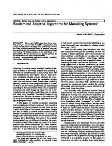
Figure 4: The spaciotemporal data set provided by Intel Berkeley Research lab presents a record of temperature data in different types of rooms throughout the lab.51 100
% Optimal Assignment
90
% Optimal VoI Collection
100
Poisson Sampling Linear Poisson Sampling Sequential Sampling Random Sampling Poisson−CGP Sampling Linear Poisson−CGP Sampling
80 70 60 50 40 30 20 10 0
0
5000
10000
90
70 60 50 40 30 20 10 0
15000
Poisson Sampling Linear Poisson Sampling Sequential Sampling Random Sampling Poisson−CGP Sampling Linear Poisson−CGP Sampling
80
0
5000
Episode
10000
15000
Episode
(a) Categorical Accuracy
(b) Percent of Maximum Score
Figure 5: The Intel Berkeley Research lab data set using (25).51 100
% Optimal VoI Collection
100
% Optimal Assignment
90 80 70 60 50 40
Poisson Sampling Linear Poisson Sampling Sequential Sampling Random Sampling Poisson−CGP Sampling Linear Poisson−CGP Sampling
30 20 10 0
0
100
200
300
400
500
600
700
800
900
1000
90 80 70 60 50 40
Poisson Sampling Linear Poisson Sampling Sequential Sampling Random Sampling Poisson−CGP Sampling Linear Poisson−CGP Sampling
30 20 10 0
0
100
200
300
Episode
400
500
600
700
Episode
(a) Categorical Accuracy
(b) Percent of Maximum Score
Figure 6: The Global Historical Climatology Network data set using (25).54
11 of 13 American Institute of Aeronautics and Astronautics
800
900
1000
VI.
Conclusion
An endurance-constrained and model-based information-theoretic approach is formulated for a UAS to ferry data between distributed UGS. The EIEIO algorithm allows the UAS to anticipate the VoI available in the distributed UGS, even in nonstationary environments, hence the optimal subset of UGS, η, may be predicted for each data-ferrying sortie. The VoI model is realized in the form of two completely Bayesian P-CGPs which do not require any a priori knowledge to implement. The P-CGPs and Poisson process approaches are incorporated into EIEIO and compared on simulated and real-world data sets. Furthermore, an optimal sampling scheme is available when there is a known sample cost for each UGS.
Acknowledgements This work was sponsored in part by Department of Energy Award Number DE-FE0012173 and the Air Force Office of Scientific Research Award Number FA9550-14-1-0399.
References 1 Bellini, A., Lu, W., Naldi, R., and Ferrari, S., “Information driven path planning and control for collaborative aerial robotic sensors using artificial potential functions,” American Control Conference (ACC), 2014 , IEEE, 2014, pp. 590–597. 2 Carfang, A. J., Frew, E. W., and Kingston, D. B., “A Cascaded Approach to Optimize Aircraft Trajectories for Persistent Data Ferrying,” AIAA Gui, 2013. 3 Celik, G. D. and Modiano, E., “Dynamic vehicle routing for data gathering in wireless networks,” Decision and Control (CDC), 2010 49th IEEE Conference on, IEEE, 2010, pp. 2372–2377. 4 Di Francesco, M., Das, S. K., and Anastasi, G., “Data collection in wireless sensor networks with mobile elements: A survey,” ACM Transactions on Sensor Networks (TOSN), Vol. 8, No. 1, 2011, pp. 7. 5 Pearre, B. and Brown, T. X., “Model-Free Trajectory Optimisation for Unmanned Aircraft Serving as Data Ferries for Widespread Sensors,” Remote Sensing, Vol. 4, No. 10, 2012, pp. 2971–3005. 6 Shah, R. C., Roy, S., Jain, S., and Brunette, W., “Data mules: Modeling and analysis of a three-tier architecture for sparse sensor networks,” Ad Hoc Networks, Vol. 1, No. 2, 2003, pp. 215–233. 7 Sugihara, R. and Gupta, R. K., “Improving the data delivery latency in sensor networks with controlled mobility,” Distributed Computing in Sensor Systems, Springer, 2008, pp. 386–399. 8 Sugihara, R. and Gupta, R., “Speed control and scheduling of data mules in sensor networks,” ACM Transactions on Sensor Networks (TOSN), Vol. 7, No. 1, 2010, pp. 4. 9 SUGIHARA, R. and GUPTA, R. K., “Path Planning of Data Mules in Sensor Networks,” . 10 Bhadauria, D., Tekdas, O., and Isler, V., “Robotic data mules for collecting data over sparse sensor fields,” Journal of Field Robotics, Vol. 28, No. 3, 2011, pp. 388–404. 11 He, L., Pan, J., and Xu, J., “A progressive approach to reducing data collection latency in wireless sensor networks with mobile elements,” Mobile Computing, IEEE Transactions on, Vol. 12, No. 7, 2013, pp. 1308–1320. 12 Lau, H. C., Yeoh, W., Varakantham, P., Nguyen, D. T., and Chen, H., “Dynamic stochastic orienteering problems for risk-aware applications,” arXiv preprint arXiv:1210.4874 , 2012. 13 Levin, L., Efrat, A., and Segal, M., “Collecting data in ad-hoc networks with reduced uncertainty,” Ad Hoc Networks, Vol. 17, 2014, pp. 71–81. 14 Li, K., Shen, C.-C., and Chen, G., “Energy-constrained bi-objective data muling in underwater wireless sensor networks,” Mobile Adhoc and Sensor Systems (MASS), 2010 IEEE 7th International Conference on, IEEE, 2010, pp. 332–341. 15 Mu, B., Chowdhary, G., and How, J. P., “Value-of-information aware active task assignment,” SPIE Defense, Security, and Sensing, International Society for Optics and Photonics, 2013, pp. 87460P–87460P. 16 Somasundara, A. A., Ramamoorthy, A., and Srivastava, M. B., “Mobile element scheduling with dynamic deadlines,” Mobile Computing, IEEE Transactions on, Vol. 6, No. 4, 2007, pp. 395–410. 17 Yu, J., Aslam, J., Karaman, S., and Rus, D., “Optimal Tourist Problem and Anytime Planning of Trip Itineraries,” arXiv preprint arXiv:1409.8536 , 2014. 18 Yu, J., Karaman, S., and Rus, D., “Persistent Monitoring of Events with Stochastic Arrivals at Multiple Stations,” arXiv preprint arXiv:1309.6041 , 2013. 19 Allamaraju, R., Kingravi, H., Axelrod, A., Chowdhary, G., Grande, R., How, J. P., Crick, C., and Sheng, W., “Human Aware UAS Path Planning in Urban Environments using Nonstationary MDPs,” . 20 Anastasi, G., Conti, M., and Di Francesco, M., “Data collection in sensor networks with data mules: An integrated simulation analysis,” Computers and Communications, 2008. ISCC 2008. IEEE Symposium on, IEEE, 2008, pp. 1096–1102. 21 Da Silva, J. E., Lucani, D. E., Baliyarasimhuni, S., and De Sousa, J. B., “Trajectory optimization for data retrieval applications: it is all about where/who loads the mule,” Navigation, Guidance and Control of Underwater Vehicles, Vol. 3, 2012, pp. 210–216. 22 Garg, S. and Ayanian, N., “Persistent Monitoring of Stochastic Spatio-temporal Phenomena with a Small Team of Robots,” Proceedings of Robotics: Science and Systems, Berkeley, USA, July 2014. 23 Sujit, P., Lucani, D., and Sousa, J., “Joint route planning for UAV and sensor network for data retrieval,” Systems Conference (SysCon), 2013 IEEE International, IEEE, 2013, pp. 688–692.
12 of 13 American Institute of Aeronautics and Astronautics
24 Mu, B., Chowdhary, G., and How, J., “Efficient distributed sensing using adaptive censoring-based inference,” Automatica, 2014. 25 O’Connor, D., Time-correlated single photon counting, Academic Press, 1984. 26 Zwanzig, R., “Time-correlation functions and transport coefficients in statistical mechanics,” Annual Review of Physical Chemistry, Vol. 16, No. 1, 1965, pp. 67–102. 27 Comte-Bellot, G. and Corrsin, S., “Simple Eulerian time correlation of full-and narrow-band velocity signals in gridgenerated,isotropicturbulence,” Journal of Fluid Mechanics, Vol. 48, No. 02, 1971, pp. 273–337. 28 Levesque, D., Verlet, L., and K¨ urkijarvi, J., “Computer” Experiments” on Classical Fluids. IV. Transport Properties and Time-Correlation Functions of the Lennard-Jones Liquid near Its Triple Point,” Physical Review A, Vol. 7, No. 5, 1973, pp. 1690. 29 Hardy, J., De Pazzis, O., and Pomeau, Y., “Molecular dynamics of a classical lattice gas: Transport properties and time correlation functions,” Physical review A, Vol. 13, No. 5, 1976, pp. 1949. 30 Lee, E. W., Wei, L., Amato, D. A., and Leurgans, S., “Cox-type regression analysis for large numbers of small groups of correlated failure time observations,” Survival analysis: state of the art, Springer, 1992, pp. 237–247. 31 Anastasi, G., Conti, M., Di Francesco, M., and Passarella, A., “Energy conservation in wireless sensor networks: A survey,” Ad Hoc Networks, Vol. 7, No. 3, 2009, pp. 537–568. 32 Loredana, A., “An information-theoretic approach for energy-efficient collaborative tracking in wireless sensor networks,” EURASIP Journal on Wireless Communications and Networking, Vol. 2010, 2010. 33 Martinez-de Dios, J., Lferd, K., de San Bernab´ e, A., N´ un ˜ez, G., Torres-Gonz´ alez, A., and Ollero, A., “Cooperation between uas and wireless sensor networks for efficient data collection in large environments,” Journal of Intelligent & Robotic Systems, Vol. 70, No. 1-4, 2013, pp. 491–508. 34 Tunca, C., Isik, S., Donmez, M., and Ersoy, C., “Distributed Mobile Sink Routing for Wireless Sensor Networks: A Survey,” 2014. 35 Zhao, F., Shin, J., and Reich, J., “Information-driven dynamic sensor collaboration,” Signal Processing Magazine, IEEE , Vol. 19, No. 2, 2002, pp. 61–72. 36 Zhao, W., Ammar, M., and Zegura, E., “A message ferrying approach for data delivery in sparse mobile ad hoc networks,” Proceedings of the 5th ACM international symposium on Mobile ad hoc networking and computing, ACM, 2004, pp. 187–198. 37 Le Ny, J., Zavlanos, M. M., and Pappas, G. J., “Resource allocation for signal detection with active sensors,” Decision and Control, 2009 held jointly with the 2009 28th Chinese Control Conference. CDC/CCC 2009. Proceedings of the 48th IEEE Conference on, IEEE, 2009, pp. 8561–8566. 38 Feillet, D., Dejax, P., and Gendreau, M., “Traveling salesman problems with profits,” Transportation science, Vol. 39, No. 2, 2005, pp. 188–205. 39 Adams, R. P., Murray, I., and MacKay, D. J., “Tractable nonparametric Bayesian inference in Poisson processes with Gaussian process intensities,” Proceedings of the 26th Annual International Conference on Machine Learning, ACM, 2009, pp. 9–16. 40 Ding, M., He, L., Dunson, D., and Carin, L., “Nonparametric Bayesian segmentation of a multivariate inhomogeneous space-time Poisson process,” Bayesian analysis (Online), Vol. 7, No. 4, pp. 813. 41 Zhou, Z., Matteson, D. S., Woodard, D. B., Henderson, S. G., and Micheas, A. C., “A Spatio-Temporal Point Process Model for Ambulance Demand,” arXiv preprint arXiv:1401.5547 , 2014. 42 Møller, J., Syversveen, A. R., and Waagepetersen, R. P., “Log gaussian cox processes,” Scandinavian journal of statistics, Vol. 25, No. 3, 1998, pp. 451–482. 43 Gunter, T., Lloyd, C., Osborne, M. A., and Roberts, S. J., “Efficient Bayesian Nonparametric Modelling of Structured Point Processes,” arXiv preprint arXiv:1407.6949 , 2014. 44 Frost, V. S. and Melamed, B., “Traffic modeling for telecommunications networks,” Communications Magazine, IEEE , Vol. 32, No. 3, 1994, pp. 70–81. 45 Paxson, V. and Floyd, S., “Wide area traffic: the failure of Poisson modeling,” IEEE/ACM Transactions on Networking (ToN), Vol. 3, No. 3, 1995, pp. 226–244. 46 Novic, B., “Bayes sequential estimation of a Poisson rate: a discrete time approach,” The Annals of Statistics, 1980, pp. 840–844. 47 Karagiannis, T., Molle, M., Faloutsos, M., and Broido, A., “A nonstationary Poisson view of Internet traffic,” INFOCOM 2004. Twenty-third AnnualJoint Conference of the IEEE Computer and Communications Societies, Vol. 3, IEEE, 2004, pp. 1558–1569. 48 Fraser, C. S., Bertuccelli, L. F., Choi, H.-L., and How, J. P., “A Hyperparameter Consensus Method for Agreement Under Uncertainty,” Automatica, Vol. 48, No. 2, February 2012, pp. 374–380. 49 El-Sayyad, G. and Freeman, P., “Bayesian sequential estimation of a Poisson process rate,” Biometrika, Vol. 60, No. 2, 1973, pp. 289–296. 50 Csat´ o, L. and Opper, M., “Sparse on-line Gaussian processes,” Neural computation, Vol. 14, No. 3, 2002, pp. 641–668. 51 Bodik, P., Hong, W., Guestrin, C., Madden, S., Paskin, M., and Thibaux, R., “Intel Lab Data,” Tech. rep., Feb. 2004. 52 Gelman, A., Carlin, J. B., Stern, H. S., Dunson, D. B., Vehtari, A., and Rubin, D. B., Bayesian data analysis, CRC press, 2013. 53 Hershey, J. R. and Olsen, P. A., “Approximating the Kullback Leibler Divergence Between Gaussian Mixture Models.” ICASSP (4), 2007, pp. 317–320. 54 Lawrimore, J. H., Menne, M. J., Gleason, B. E., Williams, C. N., Wuertz, D. B., Vose, R. S., and Rennie, J., “An overview of the Global Historical Climatology Network monthly mean temperature data set, version 3,” Journal of Geophysical Research: Atmospheres (1984–2012), Vol. 116, No. D19, 2011.
13 of 13 American Institute of Aeronautics and Astronautics