Adaptive Algorithms for Radar Detection of

[2]

[3]

[4]

[5]

[6]

[7]

[8]

[9]

[10]

[11]

[12]

[13]

[14]

Sauer, T., and Schroth, A. (1995) Robust range alignment algorithm via Hough transform in an ISAR imaging system. IEEE Transactions on Aerospace and Electronic Systems, 31, 3 (July 1995), 1173—1177. Li, X., Liu, G., and Ni, J. (1999) Autofocusing of ISAR images based on entropy minimization. IEEE Transactions on Aerospace and Electronic Systems, 35, 4 (Oct. 1999), 1240—1251. Wehner, D. R. (1994) High Resolution Radar (2nd ed.). Boston: Artech House, 1994. Ausherman, D. A., Kozma, A., Walker, J. L., Jones, H. M., and Poggio, E. C. (1984) Development in radar imaging. IEEE Transactions on Aerospace and Electronic Systems, 20, 4 (July 1984), 363—400. Prickett, M. J., and Chen, C. C. (1980) Principle of inverse synthetic aperture radar (ISAR) imaging. IEEE EASCON Record, 1980, 340—345. Pastina, D., Farina, A., Gunning, J., and Lombardo, P. (1998) Two-dimensional super-resolution spectral analysis applied to SAR images. IEE Proceedings of Radar, Sonar and Navigation, 145, 5 (Oct. 1998), 281—290. Chen, V. C. (1998) Joint time-frequency transform for radar range-doppler imaging. IEEE Transactions on Aerospace and Electronic Systems, 34, 2 (Apr. 1998), 486—499. Eichel, P. H., Ghiglia, D. C., and Jakowatz, C. V. (1989) Speckle processing method for synthetic aperture radar phase correction. Optics Letters, 14, 1 (Jan. 1989), 1—5. Wahl, D. E., Eichel, P. H., Ghiglia, D. C., and Jakowatz, C. V. (1994) Phase gradient autofocus–A robust tool for high resolution SAR phase correction. IEEE Transactions on Aerospace and Electronic Systems, 30, 3 (July 1994), 827—835. Barbarossa, S., and Farina, A. (1990) A novel procedure for detecting and focusing moving objects with SAR based on the Wigner-Ville distribution. In Proceedings of IEEE International Radar Conference, 1990, 44—50. Berizzi, and Cosini, G. (1996) Autofocusing of inverse synthetic radar images using contrast optimization. IEEE Transactions on Aerospace and Electronic Systems, 32, 3 (July 1996), 1191—1197. Bocker, R. P., Henderson, T. B., Jones, S. A., and Frieden, B. R. (1991) A new inverse synthetic aperture radar algorithm for translational motion compensation. In Proceedings of the SPIE Conference, 1991, 298—310. Steinberg, B. D., and Subbaram, H. M. (1991) Microwave Imaging Techniques. New York: Wiley, 1991.

Adaptive Algorithms for Radar Detection of Turbulent Zones in Clouds and Precipitation

The adaptive algorithm synthesis theory is used to develop new algorithms applied to radar signals in the detection of turbulent zones in clouds and precipitation. The efficiency of these new algorithms is analyzed. Simulations of weather radar signals on the one hand and modeling and testing of the processing algorithms on the other hand are performed for comparative analysis. The results demonstrate a significant superiority of the new algorithms in comparison with the widely used pulse-pair algorithm.

I. INTRODUCTION Meteorological conditions can significantly influence the flight safety of airplanes. One of the crucial meteorological factors affecting aircraft behavior is atmospheric turbulence. The overwhelming majority (97%) of dangerous turbulent zones in the atmosphere are associated with clouds and precipitation, which are detectable by radar1 [1]. Nevertheless, it does not mean that all clouds detected contain dangerous turbulent zones. We should not avoid clouds, however, but find a safe path through them. That is why weather radar is necessary as well as obligatory standard equipment of any modern aircraft. A major aspect of the operational efficiency of airborne weather radar is the reliability of turbulence detection. Detecting turbulence is difficult, because the reflectivity involved can be rather weak. Hence, noise and interference can essentially influence the reliability of the wanted information, resulting in very short detection ranges. At the same time, one of the major applications of turbulence detection is during cruise flight, at maximum airspeed. Finally, for aircraft in controlled airspace, often a significant 1 Clear air turbulence (CAT) makes only 3% of all zones of dangerous turbulence. Nevertheless it is a serious problem because of its suddenness. Due to a low concentration of hydrometeors, in most cases genuine CAT is not detectable using X-band radar. Active or passive optical systems would be better suited for these applications. Hybrid systems employing both radar and lidar or radar and interferometry would be our preferred approach to effectively detect the various manifestations of turbulence in atmosphere.

Manuscript received January 3, 2001; revised April 16 and November 15, 2002; released for publication November 15, 2002. IEEE Log No. T-AES/39/1/808688. Refereeing of this contribution was handled by L. M. Kaplan.

c 2003 IEEE 0018-9251/03/$17.00 ° CORRESPONDENCE

357

lead-time is required before turbulence avoidance maneuvers can be initiated. All these factors require large detection ranges if the turbulence detector is to be of any practical use. Available airborne radars still do not enable us to accurately detect zones of dangerous turbulence in clouds and precipitation. Therefore, at present it is necessary to use an excessively cautious decision-making strategy in order to ensure an acceptable flight safety level. This leads to an essential decrease in flight regularity, an increase in flight time, unproductive fuel expenditure, and deterioration of other air transport economic parameters. This paper is devoted to the development of new turbulence detection algorithms primarily for airborne noncoherent radar systems. However, the approach developed in this work is rather general and can be useful for different applications in weather radar engineering and radar meteorology including coherent systems as well. The paper is organized as follows. The problem is stated in Section II. Basic mathematical models are considered in Section III. Later these models are used to develop optimal algorithms under the different conditions. Gradually, these conditions become more ambiguous. Namely, in Section IV an optimal parametrical algorithm is synthesized. This algorithm provides optimum turbulence detection because all statistical information is assumed to be known. A synthesis approach, based on the turbulence detection algorithm, which is invariant to noise power, is described in Section V. Then in Section VI the synthesis using the adaptive two-sample algorithm, which is invariant to the intensity of the background scattering, is performed. Section VII gives a comparative analysis of the newly developed algorithms and the widely used pulse-pair algorithm. II. OPTIMAL TURBULENCE DETECTION: PROBLEM STATEMENT The relationship between the back-scattered radar signal parameters and the local changes in the microstructure and dynamics of atmospheric scatterers in a single-resolution volume determines the physical basis of radar detection of turbulence in clouds and precipitation. At present, two groups of informative parameters of radar signals are in use for turbulence detection. The first group includes various reflected-power characteristics related to the radar reflectivity. Statistical correlation between the radar reflectivity of clouds or precipitation and the rms velocities of the turbulent movements in them have been used for decades in the evaluation of the degree of meteorological danger to aircraft. The nature of this correlation comes from the fact that turbulence and vertical flows of air promote the growth of drops 358

and the increase in the concentration of large drops. This leads to an increase in radar reflectivity and therefore in received signal power. Thus, there are well-known radar methods of the turbulence detection based on radar reflectivity measurements, which use average values of echo-signal amplitudes [1, 2]. Averaged signal power reflected from clouds and precipitation is related statistically with dangerous zones of turbulence. However, this correlation is not strong enough to provide a tool for reliable turbulence detection. The Doppler spectrum parameters of the reflected signal belong to the second group. The Doppler spectrum depends on the distribution of radial velocities of particles weighed on their radar cross section. The theory developed in [3—5] relates spectral parameters of radar signal sequences reflected from weather objects with moving scatterers. The technique of meteorological object sounding by using ground-based weather radar to obtain information about the dynamics and microphysics of clouds and precipitation has been worked out as well [5]. Air eddies involve radar scatterers (hydrometeors) in the turbulence motion. That is why turbulence increases the velocity dispersion of scatterers. This leads to widening of the Doppler spectrum. However, at least three circumstances can decrease the relationship of turbulence intensity to the Doppler spectrum width and therefore can hamper the interpretation of experimental measurements. Firstly, the captivity of drops by air whirls is not absolute; secondly, not only turbulence but also other factors influence particle motion; and thirdly, the particle radar cross section distribution is unknown in advance. Therefore, the connection of the Doppler spectrum width with the turbulence intensity in the radar resolution volume has a statistical character that is similar to the earlier mentioned reflectivity characteristics, which belong to the first group of informative parameters. In the case of noncoherent radar, the width of the intensity fluctuation spectrum satisfying the Nyquist condition is unambiguously connected to the Doppler spectrum width [4]. Therefore, it contains information about the turbulence as well. The Doppler spectrum width is inversely related to the interperiod correlation factor. It enables us to use correlation parameters of the envelope of the echo signal in radar meteorology and avionics [5, 6]. Specifically, this idea is widely used in the so-called pulse-pair algorithm [5]. Taking into account the signal-to-noise ratio (SNR) and limited measuring time, we first discuss the performance capabilities of the pulse-pair algorithm. A radar signal reflected from clouds is a correlated random process. The correlation coefficient r between two consecutive pulses reflected from the same single radar volume (interperiod correlation factor) is a function of the turbulence intensity r = r(¾V ), where ¾V is the rms

IEEE TRANSACTIONS ON AEROSPACE AND ELECTRONIC SYSTEMS VOL. 39, NO. 1

JANUARY 2003

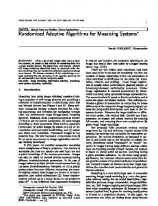
Fig. 1. Diagrams of mixture correlation factor r§ versus ¾V at different values of noise power ¾n (Ts = 0:001 s, ¸ = 0:03 m).

value of the Doppler velocity as a parameter of the turbulence intensity. The higher the turbulence intensity, the lower the correlation factor. An additive mixture of the correlated signal and uncorrelated noise is characterized by the correlation factor r§ = r°=(1 + °)

(1)

° = kR ¾V2 =¾n2

(2)

where is SNR, and kR is a dimensional factor depending on the characteristics of the radar. Substituting the model of the correlation factor [5]: r =1¡

8¼ 2 Ts2 2 ¾V = 1 ¡ CR ¾V2 ¸2

(3)

(where Ts is the pulse repetition period and ¸ is the wavelength) into (1), one can see that the correlation factor becomes a nonmonotonic function, which has a maximum value at 2 ¾V2 = ¾V0 µ ¶Á q = ¡CR kR ¾n2 + (CR kR ¾n2 )2 + CR kR2 ¾n2 CR kR2 :

(4) This corresponds to an SNR value given by s 1 °0 = ¡1 + 1 + : CR ¾n2

(5)

Starting from this value of SNR, the correlation factor decreases for increasing ¾V . That is why the pulse-pair algorithm, which actually measures the interperiod correlation factor, becomes sensitive to the increase in Doppler spectrum width and turbulence intensity only if SNR is more than °0 , as determined by expression (5). Fig. 1 shows the diagrams of the mixture correlation factor r§ versus ¾V at different values of noise power ¾n (here we set Ts = 0:001 s and ¸ = 0:03 m). Expression (5) can be used to find the necessary noise factor and receiver sensitivity in order to provide a required range of radar turbulence detection. The pulse-pair turbulence detection algorithm, which measures the correlation factor of the signal and noise mixture, should only be used in CORRESPONDENCE

measurements with SNR above the minimum value as determined by expression (5). Actually, the pulse-pair algorithm detects the decrease in the signal correlation factor. Uncorrelated noise may cause significant decorrelation in the received signal. It means that the detection threshold should then be increased. It is this circumstance that decreases greatly the efficiency of the pulse-pair algorithm at low SNR values. This leads therefore in a decrease in the range of turbulence detection. In practice, the measuring time is also a limiting factor because the statistical characteristics of sample estimates essentially depend on the number of samples. An insufficient sample number limits the reliability of any turbulence detection algorithm, which requires that the consistent estimates of informative parameters can be derived. The limited measuring time has two negative influences: firstly, it restricts the accumulation of signal power to overcome a low SNR; secondly, it restricts the time needed to obtain statistically valid estimates of the correlation factors. This short analysis shows that known methods of radar turbulence detection are based on the measuring of physically clear informative parameters. However, they do not provide the required turbulence detection quality. The signal processing algorithms in weather radars are usually not optimal. For example, the pulse-pair algorithm, which measures the correlation factor of the envelope of the mixture of weather signal and receiver noise, is not even an optimal (in any sense) estimate of the correlation factor. The usage of such estimates in weather radars is mainly based on tradition and heuristic considerations. The algorithms built on the physical considerations do not always perform best for real-life situations. On the other hand, during the development of an algorithm we are not so much interested in the real physical processes, but more in the information, which is derived from the statistical correlation between the signal parameters and the weather object characteristics. That is why we formulate the problem in terms of a statistical synthesis of turbulence detection algorithms. The purpose of this paper is to improve and clarify statistical models of the weather radar signal, and to develop optimal algorithms for the detection of dangerous turbulence in clouds and precipitation, by using the adaptive algorithm synthesis theory. Afterwards, the developed algorithms are compared with known algorithms. III. INITIAL MATHEMATICAL MODELS FOR ALGORITHM SYNTHESIS A spatial domain with hydrometeors consists of a large number of drops or crystals. They are moving randomly inside a single radar resolution volume. The statistical parameters of this motion are related 359

TABLE I Classification of Turbulence Degree of Turbulence

Negligible

Weak

Moderate

Strong

¾V , m/c

0—1.5

1.5—3

3—4.5

> 4:5

to the characteristics of atmospheric turbulence in a complicated way. In order to build turbulence detection algorithms, one must first define the mathematical models that connect signal parameters to the turbulence parameters. Such mathematical models should satisfy two basic requirements: it should 1) give an adequate description of real physical processes, 2) be a convenient analytical tool in the mathematical synthesis. These requirements are not always simultaneously satisfied. Therefore the choice of mathematical models is to some extent an art and is connected to the mathematical style of a` researcher. Our goal is achieved if the efficiency of the developed algorithm appears stable enough when certain critical parameters in the models are varied within certain limits. Otherwise, the obtained algorithms will be applicable only to a narrow class of situations where the mathematical models are adequate. We use the rms value in the velocity spread ¾v of turbulence as our primary quantitative turbulence parameter. This parameter is used in turbulence classification as defined in aeronautics [7], and shown in Table I. The classes indicated in the table correspond to those spatial scales of turbulence (about 500 m) which have the greatest effect on airplanes of intermediate size. The correlation between the turbulence characteristics and the radar signal parameters at the receiver output is used for radar turbulence detection in clouds and precipitation. In order to develop turbulence detection algorithms we assume that: 1) the spatial and temporal random behavior of scatterers is caused by turbulent motions of air, 2) the Doppler spectrum parameters are related to the scatterer motions, 3) the larger the reflected signal power, the larger the probability that turbulence is present in the cloud. Based on these assumptions, we now establish the models, which link the signal parameters to the turbulence characteristics. The reflected power P, received from an individual scatterer, can be expressed by the basic radar equation [5] and contains the radar parameters and the radar cross section of the scatterer. The amplitude of the resulting signal is a random variable. One amplitude value measured at any instant t does not contain 360

practically useful meteorological information. This is because the instantaneous signal, reflected from a volume filled with chaotically located particles, can exhibit a wide range of values. Therefore one usually ¯ ) reflected considers the average signal power P(t d from a resolution volume at distance R = ctd =2, with td as the travel time. This means that the time of averaging is much larger than the pulse repetition period Ts . Introducing the radar reflectivity Z, P¯ is represented as Z Dmax Z 2 ¯ P = C 2 jKj , Z= Ds6 N(Ds )dDs (6) R Dmin where C is the radar constant, jKj2 is a parameter related to the refraction index of the scatterer substance, and N(Ds ) is the drop size distribution with Ds being the diameter of the sphere equivalent in volume to the nonspherical scatterer. Formula (6) is correct under the condition of Rayleigh scattering, which is applicable when the largest drops have diameters significantly less than the radar wavelength, i.e., Ds ¿ ¸. This is true for cloud/raindrops detected by radar with centimeter wavelengths. More complicated formulas based on the Mie theory should be used for radar with millimeter wavelengths. For constructing a model which connects signal power parameters with turbulence parameters, we processed the data obtained by radar “Emblema” [8]. It was an X-band airborne noncoherent weather radar with typical performance characteristics (antenna beamwidth = 3:4 deg, pulse length = 1 ¹s, pulse repetition period = 1 ms). The Z values obtained during different experiments (about 700 measurements) were transformed and normalized into voltages at 30 km distance. The variance ¾2 of the weather signals is proportional to the mean ¯ therefore the data processing allowed us to power P, estimate two random variables: the rms value of the Doppler spectrum ¾V , and the rms value of amplitude variations ¾, for different clouds. The statistical processing has shown that the random values of ¾V and ¾ are dependent with a correlation factor of about 0.5. The regression dependency between ¾V and ¾ was constructed. The result obtained is in good agreement with the data of simultaneous airplane and radar measurements [1]. On average it means that, the higher the variance in amplitude of weather echoes ¾, the larger the variance turbulence movements ¾V . The established linear regression line can be written as ¾2 = kR ¾V2 :

(7)

Of course, this is just a functional relationship between statistical parameters of random values but not between the random values themselves. The simple formula (7) will be used further as an initial

IEEE TRANSACTIONS ON AEROSPACE AND ELECTRONIC SYSTEMS VOL. 39, NO. 1

JANUARY 2003

Fig. 2. Typical ACF of echo signal from Cb (boxes) and its approximation by Gaussian model (Dashed-dotted line) and exponential model (dashed line).

model which represents the first group of informative parameters as considered in Section II. Now we connect ¾V with an informative parameter of the second group. Traditionally, the Doppler spectrum g(f) of signals reflected from meteorological targets is given by a normalized Gaussian model with a mean frequency f0 and a variance in the Doppler frequency ¾f2 . The power spectrum G(F) for the amplitude detector at the fluctuation frequency F then becomes [4] µ ¶ Z 1 2 F2 G(F) = g(f)g(f + F)df = p exp ¡ 2 , 2¾F 2¼¾F ¡1 F ¸0

(8)

where ¾F2 = 2¾f2 . The normalized autocorrelation function (ACF) ½(¿ ) is Gaussian as well [9,10] and is given by ½(¿ ) = exp(¡2¼2 ¾F2 ¿ 2 ) = exp(¡4¼ 2 ¾f2 ¿ 2 ) µ ¶ ¿2 = exp ln(k) ¢ 2 ¿k

(9)

where ¿k is the correlation time at the level k (0 < k < 1). A typical ACF result of experimental weather echo measurements with a 3 cm airborne weather radar is shown in Fig. 2. The experimental data points were obtained by pulse-to-pulse registration of reflected signals coming from cumulonimbus clouds (Cb) in the Kiev region [10]. The dotted line in this figure represents an approximate ACF as modeled by a Gaussian curve with appropriate variance. Using the same experimental data, the ACF can also be approximated with other functions; e.g. by an exponential curve, shown in Fig. 2 by the dashed line. A comparison in the Doppler frequency domain has also been made. For this purpose, we first approximated the experimental ACF by the exponential and Gaussian functions. The obtained two regression equations were used to generate 2m -element vectors of real data according to each of the two approximations. Then the Fourier transform of a 2m -element vector based on the fast Fourier transform (FFT) algorithm was applied to calculate the CORRESPONDENCE

Fig. 3. Spectra calculated for Gaussian (dotted line) and exponential (solid line) approximated ACF.

Fig. 4. Measured normalized fluctuation spectrum of echoes from Cb approximated by rational function G(F).

spectrum estimates. Results are presented in Fig. 3. We note that the spectra obtained with the exponential and Gaussian approximations of ACF are rather similar. It is interesting to compare these outcomes directly with experimental estimates of spectral signal densities coming from cumulonimbus clouds (Cb), as measured in the Kiev region. In Fig. 4, the measured normalized fluctuation spectrum of echoes from Cb is approximated by the rational function: G(F) = 1=(a + bF 2 ) with

a = 9:7883535,

(10) b = 0:0019557:

The Doppler spectrum width is related to the correlation coefficient of successive reflections. According to [5], the dependence between the interperiod correlation factor of echo-signals and the rms width of the Doppler velocity spectrum is determined by formula (3). In the first-order approximation, this equals a Gaussian spectrum [10]: r = exp(¡8¼2 Ts2 ¾V2 ¸¡2 ):

(11)

For ¸ = 0:03 m and two values of Ts , we compared (3) and (11) in Fig. 5. The upper pair of curves meet at Ts = 500 ¹s and the lower pair at Ts = 1000 ¹s; the upper curve of each pair is calculated with formula (11), and the lower curve is calculated with formula (3). The outcomes show that formula (3) works well with correlation coefficients close to one, that is, at small values of ¾V and at small pulse repetition 361

probability density of the transitions according: 2

!n (x1 , : : : , xn ; r, ¾ ) = !1 (x1 ) ¢

n Y

!(xi =xi¡1 ; r, ¾2 ):

i=2

(15) Substituting (14) and the Rayleigh distribution !1 (x) = x1 =¾ 2 exp(¡x12 =2¾ 2 ) into (15), we obtain for the multidimensional probability density function of samples x1 , : : : , xn of the envelope readings of reflections from a turbulent zone !(x1 , : : : , xn ; r, ¾2 ) Fig. 5. Correlation factor r versus rms Doppler velocity ¾v : calculation on models (3) and (11) at TS = 1000 and 500 ¹s.

periods Ts . Since we assume that this condition is satisfied, we use (3) in the following. Together with (7), the relationship between the informative radar signal parameters and the weather object characteristics has been described. For mathematical convenience, we want to make use of the rational approximation (10) for G(F). As is well known, such a rational spectrum corresponds to an exponential correlation function. We now describe the narrowband process with the correlation function B(¿ ) = ¾2 e¡¯j¿ j cos !0 ¿

(12)

as a model of reflected radar signals coming from a turbulent zone. The expression (7) yields the received power variance; !0 is the radar carrier frequency. The parameter ¯ can be calculated assuming a stochastic process with a Gaussian correlation function or a stochastic process with an exponential correlation function that has the same correlation coefficients of the quadrature components. From (3) we know that µ ¶ 1 8¼ 2 ¾V2 Ts2 ¯ = ¡ ln 1 ¡ : (13) Ts ¸2 For operational use we suppose that the new algorithm for turbulence detection should work with samples of the signal envelope after the linear detector. In accordance with [15], the envelope of a narrowband Gaussian process with correlation function (12) is a Markovian process with correlation function B(¿ ) = ¾2 e¡¯j¿ j and with a conditional probability density of the transition i ¡ 1 to i " # 2 2 2 x + x r x i !(xi =xi¡1 ; r, ¾2 ) = 2 i 2 exp ¡ 2i¡1 2 ¾ (1 ¡ r ) 2¾ (1 ¡ r ) · ¸ rx x £ I0 2 i i¡12 (14) ¾ (1 ¡ r ) where r is the correlation coefficient of adjacent readings. The n-dimensional probability density function of samples x1 , : : : , xn of a Markovian process is completely determined by the one-dimensional probability density !1 (x) and the conditional 362

# " n 2 + xi2 r2 xi¡1 x1 ¡x2 =2¾2 Y xi = 2e 1 exp ¡ 2 ¾ ¾2 (1 ¡ r2 ) 2¾ (1 ¡ r2 ) i=2 · ¸ rxi xi¡1 £ I0 2 xi > 0, i = 1, : : : , n: ¾ (1 ¡ r2 )

(16)

First the statistical model (16) together with (3) and (7) will be used to synthesize the turbulence detection algorithms and then the efficiency of the developed algorithms is discussed. IV. PARAMETRICAL ALGORITHM The problem of detecting dangerous turbulent zones can be formulated as testing the parametrical hypothesis H1 : dangerous turbulence is present against the parametrical alternative H0 : dangerous turbulence is absent. The logarithm of the likelihood ratio determines the structure of the decision rule for the competing hypotheses · ¸ ! (x , : : : , xn ; ¾1 , r1 ) ¸(x1 , : : : , xn ) = ln 1 1 (17) !0 (x1 , : : : , xn ; ¾0 , r0 ) where !1 (x1 , : : : , xn ; ¾1 , r1 ) is the multidimensional probability density distribution under the hypothesis H1 and !0 (x1 , : : : , xn , ¾0 , r0 ) is the multidimensional probability density distribution under the hypothesis H0 . Substituting (16) into (17) and using the approximation ez I0 (z) ¼ p (18) 2¼z leads us to the algorithm ¸(x1 , : : : , xn ) =

n¡1 X

2 C1 xi2 + C2 xi¡1 + C3 xi xi+1 > Vp

i=2

(19) where Vp is the threshold for the decision making, and C1 = C21r02 ¡ C22r12 ; C3 = 2(C21r1 ¡ C22r0 );

C2 = C21 ¡ C22; C21 = 2¾12 (1 ¡ r12 );

C22 = 2¾02 (1 ¡ r02 ):

IEEE TRANSACTIONS ON AEROSPACE AND ELECTRONIC SYSTEMS VOL. 39, NO. 1

JANUARY 2003

The pulse-to-pulse correlation of zones with ¾V < 2 m/s (considered as nondangerous zones) can be calculated with (8) and (9); it results into r0 ¸ 0:94. Zones with ¾V > 4:5 m/s (considered as dangerous zones) are characterized by the correlation values r1 < 0:675. We choose for hypothesis H0 when ¾V = ¾0 = 1 m/s and for hypothesis H1 when ¾V = ¾1 = 4:5 m/s, meaning that ¾1 =¾0 = 4:5. For the above-mentioned classification of turbulent zones (harmless versus dangerous) we derive the quantitative values C1 , C2 , C3 , meaning that the parametrical algorithm (15) is fully determined to be used in the analysis of all kinds of input data. V. ALGORITHM INVARIANT TO NOISE POWER For a given reflectivity of clouds or precipitation, the power of the echo signal depends on the distance between the radar and the reflecting volume. In order to assure a constant false alarm probability, the threshold of decision-making Vp in the parametrical algorithm (19) should be changed with distance. Another way to stabilize false alarm probability consists of applying various automatic gain controls, which have to be fast and integrated either in the radio frequency part or in the intermediate frequency part of the receiver by means of logarithmic amplifiers. This section leads to an algorithm for turbulence detection which is invariant to the echo-signal power. We start with the probability density function and the likelihood ratio given in (16) and (17), respectively. To synthesize a detection algorithm that is invariant (with respect to signal power), we consider the likelihood ratio for the competing hypotheses averaged over all possible power values of the parameter. In other words, we introduce ¸(x1 , : : : , xn ) =

Z

1

!1 (x1 , : : : , xn , Ã, r1 )dÃ

,Z

0

1

!0 (x1 , : : : , xn , Ã, r0 )dÃ

0

(20) 2 where à = ¾ is the scale parameter that equals the reflected signal power. Substituting (16) into (20) and making use of approximation (18), we derive the algorithm: P P (1 + r0 ) ni=1 xi2 ¡ 2r0 ni=2 xi xi¡1 ¸(x1 , : : : , xn ) = Pn r1 1 + r1 Pn 2 xx i=1 xi ¡ 2 2 2(1 ¡ r1 ) (1 ¡ r1 ) i=2 i i¡1 > Vp :

(21)

It can be proven that statistics ¸(x1 , : : : , xn ) given by (21) is monotonic in the variable , n n X X 2 ³= xi xi xi¡1 : i=1

CORRESPONDENCE

i=2

Therefore, algorithm (21) has also been satisfied when we introduce the decision rule , n n X X xi2 xi xi¡1 > Vp0 (22) i=1

i=1

which is easier to use in applications. VI. TWO-SAMPLE ALGORITHM INVARIANT TO THE INTENSITY OF BACKGROUND SCATTERING The invariant one-sample algorithm (22) is not sensitive to the echo-signal power and only depends on the correlation coefficient during turbulence measurements. Additional information originating from background (Earth surface) scattering or from other fixed reflectors in the radar volume can be used to construct the so-called two-sample decision rule. Such an algorithm uses two samples: a signal sample which contains the echo signal from a turbulent zone and a learning sample y1 , : : : , yn , containing the background echo signal only. The hypothesis H0 specifies the situation in which both the signal sample and the learning sample belongs to the same distribution (16) with unknown variance ¾2 and correlation coefficient r = r0 . The hypothesis H1 still assumes distribution (16) to be valid, however, now with the variance ¾c2 = ¾ 2 (1 + °) and the correlation coefficient r = r1 (°) < r0 . Factor ° ¸ 0 determines the change in distribution (16) resulting from the change from hypothesis H0 to H1 . In accordance with the generalized empirical Bayesian technique [13, 14] the structure of the two-sample decision rule may be written as ¸(x1 , : : : , xn , y1 , : : : , yn ) R1 ! (x , : : : , xn , Ã, r1 )!0 (y1 , : : : , yn , Ã, r0 )dà = R01 1 1 0 !0 (x1 , : : : , xn , Ã, r0 )!0 (y1 , : : : , yn , Ã, r0 )dà (23) 2

where ª = ¾ corresponds to the reflected signal power; !0 and !1 are the density distributions in the hypotheses H0 and H1 , respectively. With (23) we may obtain an expression for the two-sample algorithm ¸(x1 , : : : , xn , y1 , : : : , yn ) > Vp with Vp as threshold level. Substituting probability density function expression (16) into (23), including the values of informative parameters ¾c and r in the corresponding hypotheses H0 and H1 , using (18), and executing the integration, we finally may find the statistics of the two-sample algorithm: ¸(x1 , : : : , xn , y1 , : : : , yn ) =

C1

Pn

Pn 2 Pn Pn y ) ¡ 2r0 ( i=2 xi xi¡1 + i=2 yi yi¡1 ) i=1 i Pn 2 Pn Pn

x2 + i=1 i n x2 + C2 i=1 i

(1 + r0 )(

P

y i=1 i

+ C3

xx i=2 i i¡1

+ C4

yy i=2 i i¡1

(24) 363

with 1 + r1 ; 2(1 ¡ r12 )(1 + °) r1 C3 = ¡ ; 2 (1 ¡ r1 )(1 + °) C1 =

1 + r0 ; 2(1 ¡ r02 ) r0 C4 = : (1 ¡ r02 )

C2 =

The turbulent zone can now be detected by comparing the statistics ¸(x1 , : : : , xn , y1 , : : : , yn ) determined by (24) with the decision threshold Vp . VII. COMPARATIVE ANALYSIS OF THE ALGORITHM EFFICIENCY The model of radar returns from turbulent weather formations is based on principles defined in Section III. Reflections from turbulent zones are characterized by a narrowband random process, of which the envelope is a Markovian random process with a Rayleigh density of probability distribution and exponential ACF. Dangerous weather formations are characterized by an increased reflectivity factor and stronger turbulence that result in an increase of the signal power and widening of the Doppler spectrum. The amplitude fluctuations are determined by the variance of a Gaussian process at the input of the detector and by the interperiod correlation coefficient (pulse-to-pulse correlation) as described in (7) and (3), respectively. Assuming that at time t = ti the signal x(ti ) consists of an additive mix of receiver noise and reflections from the turbulent zone, we can write x(ti ) = U(ti ) cos(!0 ti + ') + ´i

(25)

where !0 is the carrier frequency, and ´i describes the Gaussian noise. The envelope of (25) is a Rayleigh distributed random value. For a statistical modeling of the envelope of the signal, we write q i = 1, : : : , n xi = (´1i + A(ti ))2 + (´2i + B(ti ))2 , (26) where ´1i , ´2i are Gaussian uncorrelated numbers with zero mean and variances equal to the noise variance, and A(ti ) and B(ti ) are the quadrature components of the reflected signal. They represent Gaussian processes with zero means and variances as defined by (7). The correlation between successive measurements of the quadrature components depends on the rms of the turbulent velocity and is specified by (3). Sequences A(ti ), B(ti ), i = 1, : : : , n have the correlation coefficient r and are determined (after exponential smoothening) by p A(ti ) = rA(ti¡1 ) + (1 ¡ r2 )´i cos 'i (27) p B(ti ) = rB(ti¡1 ) + (1 ¡ r2 )´i sin 'i where ´i is a sequence of independent Rayleigh numbers with the scale parameter ¾´2 = kR ¾v2 ; 'i is a 364

random phase which is distributed uniformly in the interval 0 : : : 2¼. This model is in good agreement with the experiments. A simulator tool which is capable of calculating the efficiency of the turbulence detection has been developed. The software contains two major blocks. Block 1 generates echo-signal samples from turbulent zones based on algorithms (26) and (27). Block 2 executes the signal processing, and implements different turbulence detection algorithms according to expressions (19), (21), and (24), as well as the algorithm based on a direct evaluation of the sample pulse-to-pulse correlation. The last algorithm used for comparison and known as the pulse-pair algorithm, and is widely applied in weather radars. For the evaluation of pulse-to-pulse correlation, we use a sample correlation coefficient calculated via à n !2 , n à n !2 n¡1 1X 1X 1X 1X r¤ =

n

i=1

xi xi+1 ¡

n

xi

i=1

n

i=1

xi2 ¡

n

xi

:

i=1

(28) Turbulent zone detection by the pulse-pair algorithm is implemented by comparing the statistics (28) with a decision threshold. The detection characteristics are evaluated by means of the Monte-Carlo method. The number of trials for the construction of each point of the detection characteristics is 10,000. The detection threshold was set to provide the required value of the false alarm probability F under the condition of rms turbulence velocities, ¾V = 1 m/s. If ¾n2 = 0:1 and kR = 1, Fig. 1 learns that the pulse-pair algorithm can give useful information starting from ¾V . This rms level corresponds to negligible turbulence (Table I). First, the simulation was done for large SNR, ¾2 =¾n2 À 1, and the noise influence can then be neglected. Such conditions are typical for airborne weather radar when it observes a cumulonimbus cloud at the range R = 30 km as mentioned in Section III for the radar “Emblema.” Under these conditions, factor kR in (3) equals approximately 1 W¢s2 =m2 . This simulation condition was chosen as a more advantageous one for the pulse-pair algorithm, because we can see in Fig. 1 that this algorithm loses its efficiency at small SNR. The reliability of turbulence detection was calculated for different numbers of samples including rather small ones, which is important for operational weather radars particularly for airborne radars. The following sample sizes have been adopted: N = 8, 16, 32, 64, 128. The detection threshold was set to provide the given value of false alarm probability under the condition of negligible turbulence: ¾V = 1 m/s. The following values of false alarm probability were adopted: F = 0:1; 0.01; 0.001. We emphasize again that the comparative efficiency analysis of different algorithms was of primary interest in this

IEEE TRANSACTIONS ON AEROSPACE AND ELECTRONIC SYSTEMS VOL. 39, NO. 1

JANUARY 2003

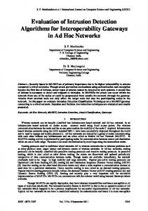
Fig. 6. Curves of turbulence detection D at false alarm probability F = 0:01 and sample size N = 16 in the case of negligible receiver noise. Curve 1 corresponds to the pulse-pair algorithm (28); 2, invariant algorithm (21); 3, adaptive algorithm (24); 4, parametrical algorithm (19).

Fig. 8. Curves of turbulence detection probability D at false alarm probability F = 0:001 and sample size N = 32 in the case of negligible receiver noise.

Fig. 9. Threshold value ¾VTh versus sample size N at false alarm probability F = 0:1 and the detection probability D = 0:9. Fig. 7. Curves of turbulence detection probability D at false alarm probability F = 0:01 and sample size N = 32 in the case of negligible receiver noise.

research. The characteristics of turbulence detection D are shown in Fig. 6 for the false alarm probability F = 0:01 and the sample size N = 16. Fig. 7 shows similar characteristics for F = 0:01 and N = 32, and Fig. 8 for F = 0:001 and N = 32. Curves marked by number 1 show the efficiency of the pulse-pair algorithm (28), curves marked by number 2 correspond to the invariant algorithm (21), number 3 to the adaptive two-sample algorithm (24), and number 4 to the parametrical algorithm (19). Each point on the curve of turbulence detection characteristic D(¾V ) determines the conditional probability of rejecting hypothesis2 “H0 : ¾V = 1 m/s” when the signal is affected by a turbulence characterized by ¾V . Hence, such turbulence detection characteristic D(¾V ) enables us to determine the conditional probability of accepting the hypothesis “H1 : ¾V = current value of ¾V .” The mark ¾VTh in Fig. 6(a) indicates (as an example) the threshold value of the rms turbulent velocity, at which algorithm (19) ensures a detection probability D = 0:8. Such a threshold value ¾VTh can be determined at different D, F, and N for each algorithm. In Fig. 9, the relationship between the threshold value ¾VTh and sample size N is shown at false alarm probability F = 0:1 for all algorithms. The curves enable us to determine the needed sample size at a given false alarm probability F and threshold value ¾VTh for each of the considered algorithms.

2 The hypotheses accepted at the stage of synthesizing detection algorithms should not necessarily coincide with those at the simulation or under the operational conditions [15].

CORRESPONDENCE

Fig. 10. Curves of turbulence detection probability D at SNR = 20 dB (N = 16, F = 0:1).

Further, the efficiency analysis has been done for the case where uncorrelated noise is present. At the simulation of the echo-signal, uncorrelated noise was added to the reflections from the weather objects. The decision-making threshold was again calculated for given false alarm probability F at a negligible turbulence, ¾V = 1 m/s. The characteristics of the turbulence detection D for N = 16, F = 0:1, and different noise levels are shown in Figs. 10 and 11. The presence of uncorrelated noise requires an increase in the decision-making threshold and, accordingly, it decreases the efficiency of the detection algorithms. Nevertheless, these results show that the efficiency of the algorithms decreased much less than that of the pulse-pair algorithm, which drops almost to zero if SNR becomes 10 dB or less (e.g., ¾n2 = 0:1 and ¾V = 1 m/s in (2) at kR = 1). The algorithms (except algorithm (21), which is invariant to power) take into account two characteristics of the reflected signal: the power and the pulse-to-pulse correlation factor. The pulse-pair algorithm is sensitive only to changes in the correlation factor. That is why it is very interesting to study the behavior of the algorithms in case the power (dispersion) of the reflected signal does not contain any useful information about turbulence. The 365

VIII. DISCUSSION AND CONCLUSION

Fig. 11. Curves of turbulence detection probability D at SNR = 10 dB (N = 16, F = 0:1).

Fig. 12. Detection probability versus rms turbulence velocity at constant dispersion (power) of weather echo signal.

detection characteristics under constant dispersion of weather echo-signals are shown in Fig. 12 for each of the analyzed algorithms. These outcomes show the comparative efficiency of different algorithms in case model (7) is not valid. It means that an echo-signal contains turbulence information only because of the widening in the Doppler spectrum but not because of an increase in the reflected power. Efficiency analysis of the considered algorithms for such a model illustrates that the new algorithms are more efficient in comparison with the pulse-pair algorithm even if turbulence does not influence the reflectivity factor. This important result can be explained by the fact that the structure of the new algorithms is based on statistical synthesis. It uses the information contained in the signal sample most completely, while the statistics of the pulse-pair algorithm is not optimal in this respect. During the analysis, additional simulations have been performed based on the quadratic conversion of the envelope. Then the process is characterized by an exponential distribution instead of the Rayleigh distribution. In this case, superiority of the developed algorithms was also shown. It means that the proposed algorithms are effective even in case the signal model differs from the initial models used in this synthesis. Thus, the set of presented curves enables us to evaluate the efficiency of the adaptive algorithms (21), (24), and the parametrical algorithm (19) in the detection of turbulent zones, and to compare them with the widely used pulse-pair algorithm (28) under different conditions. The research results show that the parametrical algorithm (19) is most efficient, followed by the adaptive two-sample algorithm (24) and the adaptive algorithm (21). All developed algorithms are more efficient than the existing reference algorithm (28). 366

The turbulence detection algorithms proposed here have been synthesized as optimal ones. The synthesis has been based on a new mathematical model for radar signals reflected from turbulent zones. The model developed here takes into account two important kinds of signal modifications caused by turbulence: changes in signal power and in the spectral structure of the pattern after the envelope detector. The change in the spectral composition appears as a spectrum widening and therefore as a decrease in the interperiod correlation coefficient. Ultimately, the signal is described as a Markovian narrowband random process with exponential ACF. The use of this convenient mathematical model together with a statistical synthesis technique of optimum decision rules has led to new adaptive algorithms for the detection of radar reflections from turbulent zones. Three new algorithms have been developed here: the parametrical algorithm, which assumes all statistical information known; the algorithm invariant to noise power; and the adaptive two-sample algorithm, which is invariant to the intensity of background scattering. The developed mathematical models and software enable us to analyze the synthesized turbulence detection algorithms and compare them with each other and with the known pulse-pair algorithm. For the analysis of the algorithm efficiency, the Monte-Carlo method was used. The sequence of readings of the envelope of the narrowband Gaussian random process that was simulated corresponds well to experimental data. The proposed new algorithms take into account two features: power and correlation factor. The pulse-pair algorithm uses a nonparametric estimation of the interperiod correlation coefficient and leaves out amplitude characteristics of the radio echo. The sample correlation coefficient, which is practically measured to implement the pulse-pair algorithm, is not an optimal correlation factor estimate of the envelope of the mix of weather signal and receiver noise. The wide application of such an estimate is based mostly on tradition and heuristics. Thus, it is natural that the efficiency of the synthesized algorithms exceeds that of the nonoptimum pulse-pair algorithm. An important task of the analysis was to compare all algorithms in the case when real characteristics of the signal differ from the models accepted in the synthesis. The analysis was done under the following conditions: 1) various SNR levels were used, including for the cases when the condition of large SNR was not valid; 2) exponential amplitude distribution was used instead of Rayleigh’s distribution accepted in the synthesis; 3) the power of the echo signal was determined independent of the

IEEE TRANSACTIONS ON AEROSPACE AND ELECTRONIC SYSTEMS VOL. 39, NO. 1

JANUARY 2003

turbulence intensity, that is, the power feature accepted in the synthesis did not work. The results of simulation assure that the proposed invariant algorithms are always superior to the pulse-pair algorithm. It is important to note that the synthesized algorithms are also highly efficient when the statistical model of the input signal is modified. This has been confirmed by simulating the data with Rayleigh or exponential distributions. Another positive aspect of the new algorithms is that they are more efficient than the pulse-pair algorithm even if the power of the echo signal is completely independent of the turbulence intensity. The advantages of the new algorithms are especially apparent at low SNR levels because there the pulse-pair algorithm detects a decrease of correlation factor, and uncorrelated noise causes strong decorrelation of the received signal. It means that the detection threshold must be increased in order to get the same false-alarm probability. That is why the efficiency of the pulse-pair algorithm is reduced sharply if SNR equals 10 dB or less. A similar phenomenon is characteristic for some multiple target indicator (MTI) algorithms, which are efficient only for large SNR (at comparatively small distances). Thus, the outcome of this analysis shows the high efficiency of the new algorithms. Each of them ensures a higher efficiency in comparison with known algorithms used already in weather radars, especially for a small number of samples, which is usual in practical circumstances. Existing methods and tools for radar detection of dangerous turbulence zones in the atmosphere show insufficient performance. The reason for this is the incomplete use of information contained in the echo signal. Simplicity of engineering realization, potentials of high efficiency and improved noise stability of the algorithms developed here promise wide applicability in modern airborne and airport weather radars. LEO P. LIGTHART FELIX J. YANOVSKY1 Delft University of Technology, IRCTR Mekelweg 4 2628 CD Delft The Netherlands E-mail: ([email protected]) E-mail: ([email protected]) IGOR G. PROKOPENKO National Aviation University Prospect Komarova 1 03058 Kiev, Ukraine

REFERENCES [1]

[2]

[3]

[4]

[5]

[6]

[7]

[8]

[9]

[10]

[11]

[12]

[13]

[14]

[15] 1 As

of April 2003; National Aviation University, Prospect Komarova 1, 03058 Kiev, Ukraine, E-mail: ([email protected]).

CORRESPONDENCE

Lee, J. T., and McPherson, A. (1971) Comparison of thunderstorms over Oklahoma and Malaysia based on aircraft measurements. In Proceedings of the International Conference on Atmospheric Turbulence, London, 1971, 1—13. Yanovsky, F. J. (1982) Airborne Weather Radars. Kiev: KIUCA Press, 1982, (in Russian). Gorelik, A. G., Melnichuk, Yu. V., and Chernikov, A. A. (1963) Relationship between statistical characteristics of radar signal and characteristics of dynamics and microstructure of weather object. Proceedings of CAO, 48 (1963), (in Russian). Atlas, D. (1964) Advances in radar meteorology. Advances in Geophysics, 10 (1964), 317—478. Doviak, R. J., and Zrnic, D. S. (1993) Doppler Radar and Weather Observations. New York: Academic Press, 1993. Yanovsky, F. J. (1974) The use of airborne radar to estimate the parameters of cloud turbulence. Radio Engineering & Electronic Physics, 9 (1974), 132—134. Vinnichenko, N. K., Pinus, N. Z., Shmeter, S. M., and Shur, G. N. (1968) Turbulence in Free Atmosphere. Leningrad: Gidrometeoizdat Publishers, 1968, (in Russian). Prockopenko, I. G., and Yanovsky, F. J. (1995) Integrated algorithm of hazardous turbulence areas detection with airborne radar. Signal Processing Methods in Aviation Radio and Electronic Equipment, Kiev: KIUCA Press, 1995, 29—35, (in Russian). Jenkins, G. M., and Watts, D. G. (1969) Spectral analysis and its applications. San-Francisco, CA: Holden-Day, 1969. Yanovsky, F. J. (1973) Estimation of the dispersion of turbulent component of wind velocity in thunderstorms on the measurements of correlation window of echo-signals of the conventional radar. VINITI, 7213—73Dep, 1973, (in Russian). Levin, B. R. (1982) Theoretical Basics of the Statistical Radio-Engineering (2nd ed.). Moscow: Sovetskoe Radio Publishers, 1982, (in Russian). Papoulis, A. (1984) Probability, Random Variables and Stochastic Processes (2nd ed.). New York: McGraw-Hill, 1984. Kornil’ev, E. A., Prokopenko, I. G., and Chuprin, V. M. (1989) Steady Algorithms in Automated Systems of Information Processing. Kiev: Tekhnika Publishers, 1989, (in Russian). Prokopenko, I. G. (1996) Double-choice adaptive algorithms for detection of radar signals in non-Gaussian noises. Radioelectronics and Communications Systems, 4 (1996), 18—23. Kendall, M. G,. and Stuart, A. (1967) The Advanced Theory of Statistics, vol. 2, Inference and Relationship (2nd ed.). London: Charles Griffin Publishers, 1967.

367