Simulation of Adaptive Array Algorithms for OFDM

Simulation of Adaptive Array Algorithms for OFDM and Adaptive Vector OFDM Systems by

Bing-Leung Patrick Cheung Thesis submitted to the faculty of the Virginia Polytechnic Institute and State University in partial fulfillment of the requirements for the degree of MASTER OF SCIENCE in Electrical Engineering

Approved:

Dr. Jeffrey H. Reed, Chairman

Dr. Brian D. Woerner

Dr. R. Michael Buehrer September 3rd, 2002 Blacksburg, Virginia

Keywords: Adaptive Antennas, Adaptive Algorithms, OFDM, AVOFDM Copyright 2002, Bing-Leung Patrick Cheung

Simulation of Adaptive Array Algorithms for OFDM and Adaptive Vector OFDM Systems by Bing-Leung Patrick Cheung Committee Chairman: Dr. Jeffrey H. Reed Bradley Department of Electrical Engineering

(ABSTRACT) The increasing demand for high data rate services necessitates the adoption of very wideband waveforms. In this case, the channel is frequency-selective, that is, a large number of resolvable multipaths are present in this environment and fading is not highly correlated across the band. Orthogonal frequency division multiplexing (OFDM) is well-known to be effective against multipath distortion. It is a multicarrier communication scheme, in which the bandwidth of the channel is divided into subcarriers and data symbols are modulated and transmitted on each subcarrier simultaneously. By inserting guard time that is longer than the delay spread of the channel, an OFDM system is able to mitigate intersymbol interference (ISI). Deploying an adaptive antenna array at the receiver can help separate the desired signal from interfering signals which originate from different spatial locations. This enhancement of signal integrity increases system capacity. In this research, we apply adaptive array algorithms to OFDM systems and study their performance in a multipath environment with the presence of interference. A novel adaptive beamforming algorithm based on the minimum mean-squared error (MMSE) criterion, which is referred to as frequency-domain beamforming, is proposed that exploits the characteristics of OFDM signals.

The computational complexity of frequency-domain

beamforming is also studied. Simulation results show employing an adaptive antenna array with an OFDM system significantly improves system performance when interference is present. Simulations also show that the computational complexity of the algorithm can be reduced by half without significant performance degradation. Adaptive array algorithms based on the maximum signal-to-noise ratio (MSNR) and the maximum signal-to-interference-plus-noise ratio (MSINR) criteria are also applied to adaptive vector OFDM systems (AV-OFDM). Simulation results show that the adaptive algorithm based on the MSNR criterion has superior performance in the multipath environment but performs worse than the one based on the MSINR criterion under the flat fading channel.

ACKNOWLEDGEMENTS I would like to express my sincerely gratitude to my academic advisor, Dr. Jeffrey H. Reed, for the invaluable support, guidance and encouragement to my research work in the Mobile and Portable Radio Research Group (MPRG) at Virginia Tech. I would also like to express my appreciation to my committee members, Dr. Brian D. Woerner and Dr. R. Michael Buehrer for their advice and comments on this work.

I wish to thank Fakhrul Alam for his guidance and fruitful discussion during the course of this research. I would like to thank him for sharing his expertise in adaptive array algorithms and provide his valuable advice in the simulation to me. I am grateful to all the members of the MPRG who assisted me through my thesis. I would especially like to thank Jay Tsai, James Hicks, Muhammad Ali Nizamuddin, and Gautam Deora for their help with my research. I greatly appreciate the help provided by all the MPRG staff members during my time here. I would also like to express my appreciation to my sponsors, Raytheon Company and MPRG Affiliates, for providing financial assistance for this work. Finally, I would like to thank my parents and family for their love and continuous support during my academic studies.

iii

TABLE OF CONTENTS

1 Introduction...................................................................................................................... 1 1.1

Motivation ..............................................................................................................1

1.2

Objective and Outline of Thesis ................................................................................2

2 Introduction To OFDM .................................................................................................... 3 2.1

Generation of OFDM Symbols .................................................................................3

2.2

Intersymbol and Intercarrier Interference...................................................................4

2.3

Guard Time Insertion ...............................................................................................6

2.4

Equalization and Channel Estimation........................................................................9

2.5

Effect of the Number of Subcarriers and Guard Time Duration .................................11

2.6

Calculation of OFDM Parameters ...........................................................................15

2.7

Windowing ...........................................................................................................16

2.8

Peak Power Problem..............................................................................................17

2.9

OFDM Versus Single -Carrier Modulation...............................................................19

2.10

Simulation Results.................................................................................................20 2.10.1 BER Performance in Static Multipath Environment ....................................21 2.10.2 BER Performance in Time-varying Multipath Environment.........................25

2.11

Chapter Summary..................................................................................................26

3 Fundamentals of Adaptive Antenna Arrays .................................................................... 27 3.1

Uniformly Spaced Linear Array..............................................................................27

3.2

Beamforming ........................................................................................................32

3.3

Spatial Filtering and Spatial Nyquist Sampling Theorem..........................................36

3.4

Criteria for Optimal Weights ..................................................................................38

3.5

3.4.1

Minimum Mean-Squared Error..................................................................39

3.4.2

Maximum Signal-to-Interference-plus-Noise Ratio .....................................40

Adaptive Algorithms for Beamforming ...................................................................43 3.5.1

Least-Mean-Square Algorithm ..................................................................43

3.5.2

Sample Matrix Inversion Algorithm...........................................................44

iv

3.5.3 3.6

Recursive Least-Squares Algorithm ...........................................................45

Chapter Summary..................................................................................................48

4 Adaptive Beamforming for OFDM Systems.................................................................... 49 4.1

Frequency-domain Beamforming............................................................................49

4.2

Adaptive Beamforming Algorithm Used in Simulation ............................................52

4.3

Performance in Two-ray Channel...........................................................................53

4.4

Beampattern..........................................................................................................57

4.5

System Parameters.................................................................................................59

4.6

Simulation Results.................................................................................................60

4.7

4.6.1

Flat Fading Channel..................................................................................60

4.6.2

Frequency-selective Fading Channel..........................................................62

Chapter Summary..................................................................................................69

5 Adaptive Beamforming for AV-OFDM Systems ............................................................. 70 5.1

AV-OFDM Waveform...........................................................................................70

5.2

AV-OFDM Transmitter .........................................................................................71

5.3

AV-OFDM Receiver..............................................................................................75

5.4

Adaptive Beamforming Algorithms ........................................................................76

5.5

Simulation Cases...................................................................................................81

5.6

System Parameters.................................................................................................82

5.7

Simulation Results.................................................................................................83

5.8

5.7.1

Flat Fading Channel..................................................................................84

5.7.2

Frequency-selective Fading Channel..........................................................93

Chapter Summary..................................................................................................97

6 Conclusions and Future Work ........................................................................................ 98 6.1

Conclusions ..........................................................................................................98

6.2

Future Work..........................................................................................................99

REFERENCES.................................................................................................................100 VITA ................................................................................................................................104

v

LIST OF FIGURES Figure 2.1

A 4-subcarrier OFDM transmitter……………………………………………....

4

Figure 2.2

Spectra of four orthogonal subcarriers………………………………………….

5

Figure 2.3

Spectra of four non-orthogonal subcarriers……………………………………..

6

Figure 2.4

Received OFDM symbols after passing through a multipath channel (a) without guard time, (b) with guard time………………………………………..

Figure 2.5

8

A 16QAM signal constellation diagram for a 64-subcarrier OFDM system without one-tap equalizers at the receiver.

The channel consists of two

multipaths, with the second one 6 dB lower than the first one and the delay spread is less than guard time………………………………………………….. Figure 2.6

12

16QAM signal constellation diagrams for a 64-subcarrier OFDM system with a two-ray multipath channel, the second ray being 6 dB lower than the first one. (a) Delay spread is less than guard time. (b) Delay spread is greater than guard time by 3.125% of the FFT interval. (c) Delay spread is greater than guard time by 9.375% of the FFT interval……………………………………...

Figure 2.7

13

16QAM signal constellation diagrams for three OFDM systems with different number of subcarriers in a two-ray multipath channel, the second ray being 6 dB lower than the first one. The ratios of delay spread to symbol duration are (a) 6.25%, (b) 3.125%, and (c) 1.56%………………………………………….

Figure 2.8

14

16QAM signal constellation diagrams for three OFDM systems with different number of subcarriers in a two-ray multipath channel, the second ray being 6 dB lower than the first one. The Doppler frequency of each ray is 120 Hz. (a) A 256-subcarrier OFDM system. (b) A 512-subcarrier OFDM system. (c) A 1024-subcarrier OFDM system…………………………………………………

Figure 2.9

15

Spectra for 128 subcarriers for raised cosine windowing with roll-off factors of 0, 0.025, 0.05, 0.1, and 0.5……………………………………………………...

17

Figure 2.10 BER vs. delay spread for a 64-subcarrier OFDM system with different guard time……………………………………………………………………………..

22

Figure 2.11 BER vs. number of subcarriers in a 5-multipath environment with delay spread exceeds guard time……………………………………………………………..

vi

23

Figure 2.12 Amplitude response of a two-ray multipath channel with the second multipath component arrived at four-symbol period later…………………………………

24

Figure 2.13 BER vs. Eb /No in a two-ray channel with delay spread less than guard time…... 24 Figure 2.14 BER vs. Doppler frequency in a 5-multipath channel with delay spread less than guard time………………………………………………………………….

25

Figure 2.15 BER vs. Doppler frequency in a 5-multipath channel with no guard time.…….

26

Figure 3.1

A uniformly spaced linear antenna array……………………………………….. 28

Figure 3.2

A narrowband beamformer……………………………………………………...

33

Figure 3.3

A wideband beamformer………………………………………………………..

34

Figure 3.4

A frequency-domain beamformer………………………………………………

36

Figure 4.1

The structure of an OFDM receiver using the frequency-domain beamforming approach…………………………………………………………………………

52

Figure 4.2

Channel impulse responses of the two-2-ray channels………………………….

53

Figure 4.3

Channel frequency responses for the 2-ray channels shown in Figure 4.2a and b, respectively…………………………………………………………………...

Figure 4.4

54

16QAM signal constellation diagrams for a 128-subcarrier OFDM system with the channel shown in Figure 4.2a. (a) one beamformer for one subcarrier; (b) one beamformer for two subcarriers; (c) one beamformer for four subcarriers...

Figure 4.5

56

16QAM signal constellation diagrams for a 128-subcarrier OFDM system with the channel shown in Figure 4.2b. (a) one beamformer for one subcarrier; (b) one beamformer for two subcarriers; (c) one beamformer for four subcarriers...

Figure 4.6

56

Beampatterns for the beamformers at the (a) 64-th subcarrier, (b) 128-th subcarrier, (c) 192-th subcarrier, (d) 256-th subcarrier, (e) 320-th subcarrier, (f) 384-th subcarrier, (g) 448-th subcarrier, and (h) 512-th subcarrier. The circle indicates the location of desired user and the asterisk indicates the location of jammers……………………………………………………………..

Figure 4.7

Simulation block diagram for an OFDM system using frequency-domain beamforming……………………………………………………………………

Figure 4.8

59

BER vs. Eb/No for a 512-subcarrier OFDM system with two wideband jammers located at 400 and -400 in a flat fading channel……………………….

Figure 4.9

58

61

BER vs. Eb/No for a 512-subcarrier OFDM system with two narrowband jammers located at 400 and -400 in a flat fading channel……………………….

62

Figure 4.10 BER vs. Eb/No for a 512-subcarrier OFDM system with two wideband jammers located at 600 and -600 in the COST 207 six-tap TU channel model…

vii

65

Figure 4.11 BER vs. Eb/No for a 512-subcarrier OFDM system with two wideband jammers located at 400 and -400 in the COST 207 six-tap TU channel model ...

66


66


67


68

Figure 4.15 BER vs. Eb/No for a 1024-subcarrier OFDM system with two wideband jammers located at 250 and -250 in the COST 207 six-tap TU channel model…

68

Figure 5.1

The AV-OFDM signal space……………………………………………………

71

Figure 5.2

Simulation block diagram for the AV-OFDM transmitter……………………...

71

Figure 5.3

Interleaver operation for a slot of Walsh sequences of size 1024………………

73

Figure 5.4

Interleaver operation for a slot of Walsh sequences of size 32…………………

74

Figure 5.5

Simulation block diagram for the AV-OFDM receiver…………………………

75

Figure 5.6

The receiver structure of the AV-OFDM system using the MSINR criterion….

77

Figure 5.7

The receiver structure of the AV-OFDM system using the MSNR criterion…...

80

Figure 5.8

BER vs. Eb /No for the three-wideband-jammer case with Walsh size of 1024 in a flat fading channel…………………………………………………………….

Figure 5.9

85

BER vs. Eb /No for the three-wideband-jammer case with Walsh size of 32 in a flat fading channel………………………………………………………………

85

Figure 5.10 Beampattern for the three-wideband-jammer case with Walsh size of 1024 using the SMI1 algorithm in a flat fading channel……………………………...

86

Figure 5.11 Beampattern for the three-wideband-jammer case with Walsh size of 1024 using the MSNR1 algorithm in a flat fading channel…………………………...

86

Figure 5.12 BER vs. Eb /No for the single strong-wideband-jammer case with Walsh size of 1024 in a flat fading channel……………………………………………………

88

Figure 5.13 BER vs. Eb /No for the single strong-wideband-jammer case with Walsh size of 32 in a flat fading channel………………………………………………………

88

Figure 5.14 Beampattern for the single strong-wideband-jammer case with Walsh size of 1024 using the SMI1 algorithm in a flat fading channel…………………….….

89

Figure 5.15 Beampattern for the single strong-wideband-jammer case with Walsh size of 1024 using the MSNR1 algorithm in a flat fading channel……………………..

viii

89

Figure 5.16 BER vs. Eb /No for the three-narrowband-jammer case with Walsh size of 1024 in a flat fading channel………………………………………………………….

91

Figure 5.17 BER vs. Eb /No for the three-narrowband-jammer case with Walsh size of 32 in a flat fading channel…………………………………………………………….

91

Figure 5.18 Beampattern for the three-narrowband-jammer case with Walsh size of 1024 using the SMI1 algorithm in a flat fading channel…………………….…….….

92

Figure 5.19 Beampattern for the three-narrowband-jammer case with Walsh size of 1024 using the MSNR1 algorithm in a flat fading channel…………………….……..

92

Figure 5.20 The Elliptical channel model……………………………………………………

93

Figure 5.21 BER vs. Eb /No for the three-wideband-jammer case with Walsh size of 1024 in a frequency-selective fading channel…………………………………………...

95

Figure 5.22 BER vs. Eb /No for the three-wideband-jammer case with Walsh size of 32 in a frequency-selective fading channel……………………………………………..

95

Figure 5.23 Beampattern for the three-wideband-jammer case with Walsh size of 1024 using the SMI1 algorithm in a frequency-selective channel……………………

96

Figure 5.24 Beampattern for the three-wideband-jammer case with Walsh size of 1024 using the MSNR1 algorithm in a frequency-selective channel…………………

ix

96

LIST OF TABLES Table 4.1

Spatial locations of seven wideband jammers…………………………………..

Table 4.2

Spatial locations and jamming power of two jammers with respect to the

57

power of the desired signal in the flat fading channel in the simulation of the OFDM system…………………………………………………………………..

60

Table 4.3

The COST-207 six-tap typical urban channel model…………………………...

62

Table 4.4

Parameters for the Jakes’ model………………………………………………...

63

Table 4.5

Computational complexity of the RLS algorithm and bandwidth of each subcarrier for an OFDM system with different number of subcarriers…………

Table 4.6

64

Spatial locations and jamming power of two jammers with respect to the power of the desired signal in the frequency-selective fading channel in the simulation of the OFDM system………………………………………………..

Table 5.1

64

Spatial locations and interference power of the three jammers with respect to the power of the desired signal in the simulation of the AV-OFDM system…...

81

Table 5.2

AV-OFDM signal parameters…………………………………………………..

82

Table 5.3

Parameter values for the 32-ary and 1024-ary Walsh modulation schemes…….

83

Table 5.4

Parameters of the Elliptical channel model……………………………………..

93

x

Chapter 1 : Introduction

1.1

Motivation

The focus of future fourth-generation (4G) mobile systems is to support high data rate services and to ensure seamless provisioning of services across a multitude of wireless systems and networks, from indoor to outdoor, from one air interface to another, and from private to public network infrastructure [1][2].

Higher data rates allow the deployment of multi-media

applications which involve voice, data, pictures, and video over the wireless networks. At this moment, the data rate envisioned for 4G networks is 1Gb/s for indoor and 100Mb/s for outdoor environments [3]. High data rate means the signal waveform is truly wideband, and the channel is frequency-selective from the waveform perspective, that is, a large number of resolvable multipaths are present in the environment. Orthogonal frequency division multiplexing (OFDM), which is a modulation technique for multicarrier communication systems, is a promising candidate for 4G systems since it is less susceptible to intersymbol interference introduced in the multipath environment [4]. An adaptive antenna array deployed at the receiver is able to enhance the signal integrity in an interference environment [6]. If the desired signal and the interfering signals are located at different spatial locations, an antenna array can act as a spatial filter which separates the desired signal from the interferin g signal. In the cellular environment, using an adaptive antenna can reduce the co-channel interference from other users within its own cell and the neighboring cells, thus increasing system capacity [5]. Due to its advantages, an adaptive antenna array is likely to be an integral part of the 4G systems. The application of adaptive algorithms in the antenna array for the single -carrier systems has been studied extensively.

However, there are relatively few technical papers on applying smart

antennas to OFDM systems and investigating interference suppression capability for multipath environments. The nature of modulation/demodulation on subcarriers in an OFDM system requires a new approach for implementing adaptive algorithms in the antenna array. Therefore, it is necessary to understand the fundamental principle of OFDM and to develop techniques for applying adaptive array algorithms to OFDM systems.

1

CHAPTER 1: INTRODUCTION

1.2

Objective and Outline of Thesis

The objective of this research is to apply adaptive array algorithms to an OFDM system and investigate its interference suppression capability in a multipath environment. This thesis is organized as follows. Chapter 2 introduces the fundamentals of OFDM. It covers the basic concept, the terminology, and simulation results of an OFDM system employing a single antenna under both the static and multipath fading channels. Chapter 3 introduces the fundamentals of adaptive antenna arrays. It discusses different beamformer structures and also a number of common adaptive beamforming algorithms applied in the antenna array.

Chapter 4 presents a detailed analysis of adaptive beamforming for OFDM systems. The concept of frequency-domain beamforming is introduced here. The structure of the frequency-domain beamformer is provided and the adaptive beamforming algorithm used in the simulation is explained. A study of the proposed beamforming algorithm is presented for a two-ray channel model. Finally, simulation results are provided for an OFDM system using an 8-element antenna array with two jammers under a flat fading channel and the COST-207 six tap urban channel model. Chapter 5 presents the baseband simulation model for the adaptive vector OFDM (AV-OFDM) system using an antenna array. The AV-OFDM system is a spread-spectrum communication system which uses Walsh orthogonal modulation to spread an OFDM signal. In this chapter, the waveform and the structure of the transmitter and receiver used in the simulation are described. The adaptive beamforming algorithms proposed for the AV-OFDM system are also described in detail. Finally, detailed comparisons of the BER performance of the different beamforming algorithms in various simulation cases are provided at the end of this chapter. Chapter 6 concludes the thesis and summarizes the results of the work. Areas for future work are also suggested.

2

Chapter 2 : Introduction To OFDM

Orthogonal frequency division multiplexing (OFDM) is based on the multicarrier communications technique. The idea of multicarrier communications is to divide the total signal bandwidth into number of subcarriers and information is transmitted on each of the subcarriers. Unlike the conventional multicarrier communication scheme in which spectrum of each subcarrier is non-overlapping and bandpass filtering is used to extract the frequency of interest, in OFDM the frequency spacing between subcarriers is selected such that the subcarriers are mathematically orthogonal to each other. The spectra of subcarriers overlap each other but individual subcarrier can be extracted by baseband processing. This overlapping property makes OFDM more spectral efficient than the conventional multicarrier communication scheme.

2.1

Generation of OFDM Symbols

A baseband OFDM symbol can be generated in the digital domain before modulating on a carrier for transmission. To generate a baseband OFDM symbol, a serial of digitized data stream is first modulated using common modulation schemes such as the phase shift keying (PSK) or quadrature amplitude modulation (QAM). These data symbols are then converted from serial-toparallel (S/P) before modulating subcarriers. Subcarriers are sampled with sampling rate N / Ts , where N is the number of subcarriers and Ts is the OFDM symbol duration. The frequency separation between two adjacent subcarriers is 2π / N . Finally, samples on each subcarrier are summed together to form an OFDM sample. An OFDM symbol generated by an N-subcarrier OFDM system consists of N samples and the m-th sample of an OFDM symbol is [7] N −1  2π mn  xm = ∑ X n exp  j , 0 ≤ m ≤ N −1 , N   n =0

(2.1)

where X n is the transmitted data symbol on the n-th subcarrier. Equation 2.1 is equivalent to the N-point inverse discrete Fourier transform (IDFT) operation on the data sequence with the omission of a scaling factor. It is well known [8] that IDFT can be implemented efficiently using

3

CHAPTER 2: INTRODUCTION TO OFDM inverse fast Fourier transform (IFFT). Therefore, in practice, the IFFT is performed on the data sequence at an OFDM transmitter for baseband modulation and the FFT is performed at an OFDM receiver for baseband demodulation. Finally, a baseband OFDM symbol is modulated by a carrier to become a bandpass signal and transmitted to the receiver. In the frequency domain, this corresponds to translating all the subcarriers from baseband to the carrier frequency simultaneously. Figure 2.1 shows a 4-subcarrier OFDM transmitter and the process of generating one OFDM symbol. exp( j0 n)

1st symbol

exp( j π n 2)

4th symbol

exp( j 2π f ct ) Bit Stream

PSK/ QAM

S/P

exp( jπ n)

Σ

exp( j 3π n 2)

Figure 2.1 A 4-subcarrier OFDM transmitter.

2.2

Intersymbol and Intercarrier Interference

In a multipath environment, a transmitted symbol takes different times to reach the receiver through different propagation paths. From the receiver’s point of view, the channel introduces time dispersion in which the duration of the received symbol is stretched. Extending the symbol duration causes the current received symbol to overlap previous received symbols and results in intersymbol interference (ISI). In OFDM, ISI usually refers to interference of an OFDM symbol by previous OFDM symbols.

4

CHAPTER 2: INTRODUCTION TO OFDM In OFDM, the spectra of subcarriers overlap but remain orthogonal to each other. This means that at the maximum of each subcarrier spectrum, all the spectra of other subcarriers are zero. The receiver samples data symbols on individual subcarriers at the maximum points and demodulates them free from any interference from the other subcarriers. Interference caused by data symbols on adjacent subcarriers is referred as intercarrier interference (ICI). The orthogonality of subcarriers can be viewed in either the time domain or frequency domain. From the time domain perspective, each subcarrier is a sinusoid with an integer number of cycles within one FFT interval. From the frequency domain perspective, this corresponds to each subcarrier having the maximum value at its own center frequency and zero at the center frequency of each of the other subcarriers. Figure 2.2 shows the spectra of four subcarriers in the frequency domain for the orthogonality case.

0.9 0.8 0.7 0.6 0.5 0.4 0.3 0.2 0.1 0 0

1

2

3

4 5 Subcarrier Index

6

7

8

Figure 2.2 Spectra of four orthogonal subcarriers.

The orthogonality of a subcarrier with respect to other subcarriers is lost if the subcarrier has nonzero spectral value at other subcarrier frequencies. From the time domain perspective, the corresponding sinusoid no longer has an integer number of cycles within the FFT interval. Figure 2.3 shows the spectra of four subcarriers in the frequency domain when orthogonality is lost.

5

CHAPTER 2: INTRODUCTION TO OFDM

0.9 0.8 0.7 0.6 0.5 0.4 0.3 0.2 0.1 0 0

1

2

3


6

7

8

Figure 2.3 Spectra of four non-orthogonal subcarriers.

ICI occurs when the multipath channel varies over one OFDM symbol time [9]. When this happens, the Doppler shifts on each multipath component causes a frequency offset on the subcarriers, resulting in the loss of orthogonality among them. ICI also occurs when an OFDM symbol experiences ISI. This situation can be viewed from the time domain perspective, in which the integer number of cycles for each subcarrier within the FFT interval of the current symbol is no longer maintained due to the phase transition introduced by the previous symbol. Finally, any offset between the subcarrier frequencies of the transmitter and receiver also introduces ICI to an OFDM symbol.

2.3

Guard Time Insertion

OFDM is resilient to ISI because its symbol duration is long compared with the data symbols in the serial data stream. For an OFDM transmitter with N subcarriers, if the duration of a data symbol is T’, the symbol duration of the OFDM symbol at the output of the transmitter is Tsym = T ' N .

6

(2.2)

CHAPTER 2: INTRODUCTION TO OFDM Thus if the delay spread of a multipath channel is greater than T’ but less then Tsym, the data symbol in the serial data stream will experience frequency-selective fading while the data symbol on each subcarrier will experience only flat-fading. Moreover, to further reduce the ISI, a guard time is inserted at the beginning of each OFDM symbol before transmission and removed at the receiver before the FFT operation. If the guard time is chosen such that its duration is longer than the delay spread, the ISI can be completely eliminated. Figure 2.4 illustrates the concept of guard time insertion to eliminate ISI for an OFDM symbol. In Figure 2.4a, an OFDM symbol received from the first path is interfered by the previous OFDM symbol received from the second and third paths. On the other hand, Figure 2.4b shows that the OFDM symbol received from the first path is no longer interfered by the previous OFDM symbol. However, the received symbol is still interfered by its replicas and we refer to this type of interference as self-interference. In order to preserve orthogonality among subcarriers, the guard time is inserted by cyclically extending an OFDM symbol. If the delay spread is less than the guard time, the delay spread only introduces a different phase shift for each subcarrier but does not destroy the orthogonality between subcarriers. Guard time insertion can be performed in two ways: 1. Extract a portion of an OFDM symbol at the end and append it to the beginning of the OFDM symbol. Samples after guard time insertion can be expressed as [7] x kg = x (k + N −G )N , 0 ≤ k ≤ N + G − 1 ,

(2.3)

where k is the sample index of an OFDM symbol, N is the number of subcarriers, G is the guard time duration, and ( k )N is the residue modulo N .

2. Extract a portio n of an OFDM symbol at the end and append it to the beginning, and at the same time extract a portion of the OFDM symbol at the beginning and append it to the end of the symbol. Samples after guard time insertion can be expressed as xkg = x(k + N −Tprefix )N , 0 ≤ k ≤ N + G − 1, G = Tprefix + Tpost ,

(2.4)

where Tprefix is the guard time duration appending to the beginning of the symbol and Tpost is the guard time duration appending to the end of the symbol.

7

CHAPTER 2: INTRODUCTION TO OFDM For the same guard time duration, method 1 gives the maximum delay spread tolerance since the whole guard time is contributed to eliminate ISI. Method 2 contributes only a portion of the guard time (the portion at the beginning of an OFDM symbol) to reduce ISI. Method 2 is more appropriate when win dowing is performed on an OFDM symbol to reduce the out-of-band spectrum since the roll-off regions at the two end of the symbol do not attenuate the data symbols on the subcarriers. Windowing will be explained more in detail later in the chapter.

Multipath channel

time Symbol arrives at

1 symbol duration

Direct path 1st multipath 2nd multipath

ISI

(a)

Self interference

1 symbol duration

Guard time

1 FFT duration

Symbol arrives at Direct path 1st multipath 2nd multipath

(b)

Self interference

Figure 2.4 Received OFDM symbols after passing through a multipath channel (a) without guard time, (b) with guard time.

8


2.4

Equalization and Channel Estimation

Although the guard time which has longer duration than the delay spread of a multipath channel can eliminate ISI completely, the received symbol is still interfered by its replicas received from multipath components. This corresponds to frequency-selective fading of the symbol. In order to compensate this distortion, a one-tap channel equalizer is needed for each subcarrier. At the output of FFT on the receiver side, the sample at each subcarrier is multiplied by the coefficient of the corresponding channel equalizer. The coefficient of an equalizer can be calculated based on the zero-forcing (ZF) criterion or the minimum mean-square error (MMSE) criterion [10]. The ZF criterion forces ISI to be zero at the sampling instant of each subcarrier. The coefficient of a one-tap ZF equalizer is calculated as follows: Cn =

1 , Hn

(2.5)

where H n is the channel frequency response within the bandwidth of the n-th subcarrier. The disadvantage of the ZF criterion is that it enhances noise at the n-th subcarrier if H n is small, which corresponds to spectral nulls. To make the trade off between ISI and noise, MMSE criterion is used and the coefficient of a one-tap MMSE equalizer is calculated as follows: Cn =

H n* 2 2 H n + σ noise σ symbol 2

,

(2.6)

2 2 where σ noise is the noise variance and σ symbol is the variance of source symbols. A MMSE

equalizer gives better performance than a ZF equalizer when spectral nulls are present in the channel frequency response. Equation 2.5 and 2.6 show that one needs to perform channel estimation in order to obtain weights for equalizers on individual subcarriers. Training symbols, also known as pilot symbols, are also often used to perform channel estimation. In OFDM, since equalization is performed in the frequency domain, it is the channel frequency response that must be estimated. In the multipath environment, the demodulated symbol X n on the n-th subcarrier at the output of FFT without ISI and ICI can be represented as  L −1   2π nl   Yn = ∑ H l (0)exp − j     X n + Nn ,   N    l =0

9

(2.7)

CHAPTER 2: INTRODUCTION TO OFDM where L is the number of multipath components, Nn is the FFT of the additive white Gaussian noise (AWGN) on the n-th subcarrier and H l (0) is the channel frequency response of the l-th multipath component at the zero-th frequency. To estimate the channel frequency response, pilot symbols are inserted on the subcarriers in the frequency domain, i.e., they are inserted before IFFT operation at the transmitter side. Let H n be the channel frequency response experienced by X n , i.e. L −1  2π nl  H n = ∑ H l (0)exp  − j . N   l =0

(2.8)

The channel frequency response experienced by the pilot symbol Pn on the n-th subcarrier can be estimated as Y Hˆ n = n Pn = Hn +

Nn . Pn

(2.9)

Since pilot symbols usually occupy a small amount of bandwid th for spectral efficiency, interpolation across frequency is required to estimate the channel frequency response where pilot symbols are not located. The channel frequency response at the m-th subcarrier Hˆ m can be interpolated linearly as [11] m  m Hˆ m = 1 −  Hˆ p1 + Hˆ p2 , N  N

p1 ≤ m ≤ p2 ,

(2.10)

where Hˆ p1 and Hˆ p2 are the channel frequency responses estimated by the pilot symbols on the p 1 -th and p 2 -th subcarriers. Furthermore, if the multipath channel is time-varying in nature, then interpolation across time may also require tracking the channel. To determine the minimum pilot spacing in time and frequency in OFDM, we need to find the bandwidth of the channel variation in time and frequency. These bandwidths are equal to the maximum Doppler frequency f Dmax in the time domain and the maximum delay spread τ max in the frequency domain. According to the sampling theorem, the pilot spacing in time st and frequency s f is [12]

10

CHAPTER 2: INTRODUCTION TO OFDM st ≤

sf ≤

1

(2.11)

2 f Dmax Ts

1 2τ max ∆F

,

(2.12)

where Ts is the OFDM symbol duration and ∆F is the frequency spacing between two subcarriers. Decreasing the pilot spacing improves the estimation of channel frequency response but decreases bandwidth efficiency. On the other hand, increasing the pilot spacing beyond the one specified by the sampling theorem decreases the accuracy of the channel estimation but increases the bandwidth efficiency. Hence, the chosen pilot density is a tradeoff between the performance of channel estimation and bandwidth efficiency. Moreover, besides interpolating the channel frequency response in the frequency and time domain separately, a two-dimensional interpolation can also be applied in OFDM. More detail on the two-dimensional interpolation scheme can be found in [4][12][13].

2.5

Effect of the Number of Subcarriers and Guard Time Duration

In this section, a number of signal constellation diagrams are shown for an OFDM system to study the effect of the number of subcarriers and the guard time duration on the performance of an OFDM system. 16QAM modulation scheme is used for a 64-subcarrier OFDM system with a two-ray multipath channel. The power of the second path is 6 dB lower than the first one. No noise is present at the receiver in order to have a clear idea of the influence of ISI and ICI on the system performance with respect to these two parameters. Figure 2.5 shows the 16QAM signal constellation diagram for delay spread less than guard time and no channel equalizers are implemented at the receiver. It shows that the received signal points have a circular pattern around the transmitted signal points. Self-interference moves some of the signal points over the decision boundaries and results in significant degradation in biterror-rate (BER) performance. Therefore, one-tap channel equalizers must be implemented at the FFT output to correct the amplitude and phase distortion caused by multipath distortion. The circular pattern on the signal constellation diagram can also be observed by performing circular convolution of a multipath channel and an OFDM symbol without cyclic extension. As pointed out in [10] and [29], the cyclic extension makes the linear convolution of the channel

11

CHAPTER 2: INTRODUCTION TO OFDM looks like circular convolution inherent to the discrete Fourier domain, as long as the guard time duration is longer than the delay spread of the multipath channel. 5 4 3 2 1 0 -1 -2 -3 -4 -5 -5

0

5

Figure 2.5 A 16QAM signal constellation diagram for a 64-subcarrier OFDM system without one-tap equalizers at the receiver. The channel consists of two multipaths, with the second one 6 dB lower than the first one and the delay spread is less than guard time.

Figure 2.6 shows the 16QAM signal constellation diagrams for the case of a 64-subcarrier OFDM system with one-tap equalizers at the receiver.

Figure 2.6a shows the 16QAM signal

constellation for the case of delay spread less than the guard time duration. No distortion is observed since the delay spread is shorter than the guard time and the frequency-selective fading is compensated by the one-tap equalizers. Figure 2.6b and 2.6c show the constellation diagram for the case of delay spread greater than the guard time by 3.125% and 9.375% of the FFT interval respectively. The distortion caused by ISI gets bigger as the delay spread exceeds the duration of the guard time more, resulting in higher BER.

12


6

6

6

4

4

4

2

2

2

0

0

0

-2

-2

-2

-4

-4

-4

-6 -6

-4

-2

0

2

4

6

-6 -6

(a)

-4

-2

0

2

4

6

-6 -6

-4

-2

(b)

0

2

4

(c)

Figure 2.6 16QAM signal constellation diagrams for a 64-subcarrier OFDM system with a two-ray multipath channel, the second ray being 6 dB lower than the first one. (a) Delay spread is less than guard time. (b) Delay spread is greater than guard time by 3.125% of the FFT interval. (c) Delay spread is greater than guard time by 9.375% of the FFT interval.

The influence of ISI can be reduced by increasing the duration of an OFDM symbol. To quantify the influence, we define a measure as η=

delay spread . symbol duration

(2.13)

For a given bandwidth of an OFDM signal, the symbol duration is proportional to the number of subcarriers. If η is large, a significant number of samples of individual OFDM symbols are affected by ISI and thus the system will have a high BER. On the other hand, if η is small, a small portion of the individual OFDM symbols is affected by ISI and thus the system will have a low BER. Figure 2.7 shows the signal constellation diagrams for three OFDM systems with a different number of subcarriers. The ratios of the delay spread to the OFDM symbol duration are 6.25%, 3.125%, and 1.56% respectively. The one with the smallest ratio corresponds to the largest number of subcarriers. It shows that ISI is more severe for the OFDM system with small number of subcarriers compared with the one that has a large number of subcarriers.

13

6


6

6

6

4

4

4

2

2

2

0

0

0

-2

-2

-2

-4

-4

-4

-6 -6

-4

-2

0

2

4

6

-6 -6

-4

-2

(a)

0

2

4

6

-6 -6

-4

(b)

-2

0

2

(c)

Figure 2.7 16QAM signal constellation diagrams for three OFDM systems with different number of subcarriers in a two-ray multipath channel, the second ray being 6 dB lower than the first one. The ratios of delay spread to symbol duration are (a) 6.25%, (b) 3.125%, and (c) 1.56%.

OFDM symbols with long duration are more resilient to frequency-selective fading but more sensitive to time-selective fading. Time-selective fading results in the loss of orthogonality among subcarriers. Figure 2.8 shows the 16QAM signal constellation diagrams for three OFDM systems with 256, 512, and 1024 subcarriers respectively. The two-ray channel is time-varying with each path having Doppler frequency of 120Hz. From the figure, it shows that the signal constellation diagram for the 1024-subcarriers OFDM system is more blurred than the 256subcarrier and 512-subcarrier OFDM systems. For a given signal bandwidth, the frequency spacing between subcarrie rs decreases as the number of subcarrier increases.

The small

frequency separation between two subcarriers makes them more vulnerable to the ICI due to the frequency offset introduced by the Doppler spread of the channel. The effect of the number of subcarriers and guard time duration on the system performance is summarized as follows [14]: •

For a given number of subcarriers, increasing guard time duration reduces ISI due to the decrease in delay spread relative to the symbol time, but reduces the power efficiency and bandwidth efficiency.

•

For a given signal bandwidth, increasing the number of subcarriers increases the power efficiency but also increases the symbol duration and results in a system more sensitive to Doppler spread.

14

4

6


6

6

6

4

4

4

2

2

2

0

0

0

-2

-2

-2

-4

-4

-4

-6 -6

-4

-2

0

2

4

6

-6 -6

-4

-2

(a)

0

2

4

6

-6 -6

-4

-2

(b)

0

2

4

(c)

Figure 2.8 16QAM signal constellation diagrams for three OFDM systems with different number of subcarriers in a two-ray multipath channel, the second ray being 6 dB lower than the first one. The Doppler frequency of each ray is 120Hz. (a) A 256-subcarrier OFDM system. (b) A 512subcarrier OFDM system. (c) A 1024-subcarrier OFDM system.

2.6

Calculation of OFDM Parameters

For a given bit rate R and the delay spread of a multipath channel τ, the parameters of an OFDM system can be determined as follows [4]: •

As a rule of thumb, the guard time G should be at least twice the delay spread, i.e. G ≥ 2τ .

•

(2.14)

To minimize the signal-to-noise ratio (SNR) loss due to the guard time, the symbol duration should be much larger than the guard time. However, symbols with long duration are susceptible to Doppler spread, phase noise, and frequency offset. As a rule of thumb, the OFDM symbol duration Tsym should be at least five times the guard time, i.e. Tsym ≥ 5G .

•

The frequency spacing between two adjacent subcarriers ∆f is ∆f =

•

(2.15)

1 . Tsym

(2.16)

For a given data rate R, the number of information bits per OFDM symbol Binfo is Binfo = RTsym .

15

(2.17)

6

CHAPTER 2: INTRODUCTION TO OFDM •

For a given Binfo and the number of bits per symbol per subcarrier Rsub , the number of subcarriers N is N=

Binfo Rsub

,

(2.18)

where Rsub = 2 bits/symbol/subcarrier for QPSK Rsub = 4 bits/symbol/subcarrier for 16-QAM.

•

The OFDM signal bandwidth is defined as BW = N ∆f .

(2.19)

Two observations are made from the above calculations: •

Increasing the symbol duration decreases the frequency spacing between subcarriers. Thus, for a given signal bandwidth, more subcarriers can be accommodated. On the other hand, for a given number of subcarriers, increasing the symbol duration decreases the signal bandwidth.

•

Increasing the number of subcarriers increases the number of samples per OFDM symbol. However, it does not necessary imply that the symbol duration increases. If the OFDM symbol duration remains the same, the duration between two samples decreases as a result. This implies the increase in the OFDM signal bandwidth. On the other hand, if the OFDM signal bandwidth is fixed, then increasing the number of subcarriers decreases the frequency spacing between two subcarriers, which in turn increases the symbol duration. The duration between two samples remain the same in this case.

2.7

Windowing

Phase transition on a subcarrier occurs at the boundary of an OFDM symbol if the two consecutive bits modulating on the same subcarrier have different values. Sharp phase transitions result in a slow rolloff of the out-of-band spectrum. Windowing an OFDM symbol makes the out-of-band spectrum go down more quickly. In [4], a raised-cosine window is applied to OFDM symbols and is defined as follows:

16

CHAPTER 2: INTRODUCTION TO OFDM 0 ≤ t ≤ β Ts  0.5 + 0.5cos(π + tπ /(β Ts ))  w(t ) =  1.0 , β Ts ≤ t ≤ Ts , 0.5 + 0.5cos((t − T )π /( β T )) T ≤ t ≤(1 + β )T s s  s s

(2.20)

where Ts is the OFDM symbol duration including the guard time, β is the roll-off factor, and β Ts is the overlap region of two consecutive OFDM symbols. Figure 2.9 shows the spectra for 128 subcarriers with different roll-off factors.

0 -10 -20

PSD (dB)

-30 -40

0

-50

0.025

-60 0.05 -70 0.1

-80 -90 -100

0.5 -110 -1

-0.5

0 Normalized Frequency

0.5

1

Figure 2.9 Spectra for 128 subcarriers for raised cosine windowing with roll-off factors of 0, 0.025, 0.05, 0.1, and 0.5.

2.8

Peak Power Problem

A major disadvantage of an OFDM system is its large peak-to-average power ratio (PARP) due to the summation of a large number of subcarriers coherently. As the number of subcarriers N increases, the maximum possible peak power becomes N times the average power [15]. A large value of PARP requires a wide linear region of the amplifier in order to avoid signal waveform distortion. However, an amplifier has only a certain range of linear region and beyond that is the saturation region, where the output power does not increase even though the input power

17

CHAPTER 2: INTRODUCTION TO OFDM increases substantially.

Therefore, in order to make sure that an amplifier in an OFDM

transmitter is operated in a linear region, the mean output power should be N times less than the maximum possible power. Output backoff (OBO) refers to the amount (in dB) by which the average output power is reduced from the saturation power. Large OBO results in power inefficiency of the linear amplifier. A nonlinear amplifier is power efficient but it introduces signal distortion to a certain extent. Two solutions are proposed to solve this problem. One is to improve the power efficiency of a linear amplifier, and the other one is to reduce the PARP. Methods to improve the power efficiency of a linear amplifier include amplifier linearization techniques and dc bias controlling techniques. Details of these two methods are given in the references of [16]. Methods to reduce PARP will be discussed below. The PARP reduction techniques can be divided into three categories [4]. The first one is the signal distortion techniques, which include clipping, peak windowing, and peak cancellation to reduce the peak amplitudes of an OFDM signal. Clipping sets those peak amplitudes that exceed a threshold value to a maximum desired level. The advantage of this method is simplicity and the disadvantages are the introduction of in-band distortion and out-of-band spectral leakage. To reduce the out-of-band spectral leakage, peak windowing is used. The idea is to multiply the large signal peaks with some window functions such as cosine, Kaiser, and Hamming windows such that the out-of-band spectrum decreases rapidly.

Both clipping and peak win dowing

introduce nonlinear distortion which causes out-of-band spectral leakage. Peak cancellation [17] avoids the nonlinear distortion by subtracting a reference function from the OFDM signal to reduce the peak amplitudes. One of the suitable reference functions is the sinc function. A sinc function is usually multiplied with the raised-cosine window to make sure the reference function has the same bandwidth as the OFDM signals with no extra out-of-band spectrum introduced. The second category consists of coding techniques, which excludes the OFDM symbols that have high PARP and hopefully those excluded symbols can be recovered from forward-error correction of the code set. Golay complementary sequences are considered as a good candidate to modulate an OFDM signal.

They provide good forward-error correction capabilities while

reducing the PAPR to 3 dB [18].

The third category is the scrambling techniques which

multiplies each OFDM symbol with different scrambling codes and selects the one with the smallest PAPR. There are two sub-categories. Selected mapping multiplies the data sequences on all the subcarriers with different scrambling sequences, then performs IFFT on those sequences and selects the one with the smallest PARP for transmission [19]. Partial transmit

18

CHAPTER 2: INTRODUCTION TO OFDM sequence divides the data sequences into subblocks and performs N-point IFFT on each subblock, then multiples each subblock with different scrambling rotations and finally combines all the subblocks to minimize the PAPR [20].

2.9

OFDM Versus Single-Carrier Modulation

Several papers [21][22][23][24] have investigated the performance of OFDM versus a single carrier modulation scheme. It is well known that OFDM is more effective to combat ISI compared with a single -carrier system using a time-domain equalizer, especially for channels with large delay spread. Moreover, the efficiency of FFT algorithms implemented in OFDM also makes the computational complexity much less than the time-domain equalization in a single carrier system [4]. However, for large FFT sizes, a single -carrier system employing frequencydomain equalization has much lower complexity as compared with time-domain equalization [25]. Recent papers usually compare the system performance of an OFDM system with a single carrier system employing frequency-domain equalization because the complexities are comparable. Two main issues come up from the comparison of an OFDM system with a single -carrier system. The first one is the power amplification issue. If the data sequence is modulated using PSK scheme, then the output signal has a low envelope fluctuation with a compact spectrum for a single-carrier system. For a multi-carrier system, such as OFDM, the envelope fluctuation is large. In fact, according to the central limit theorem, the real and imagery parts of an OFDM symbol are Gaussian distributed for a large number of subcarriers, making the envelope of the OFDM signal Raleigh distributed. A signal with large envelope fluctuation requires a power amplifier with large backoff, which makes the amplifier power inefficient. Therefore, the power amplifier for a single -carrier system has a good power efficiency compared with that for an OFDM system. The second issue is the impact of the channel coding to system performance. The performance of a communication system is usually measured in terms of BER for a specific SNR. Consider the case in which the channel is frequency-selective. For a single -carrier system using the frequencydomain equalization scheme, once the channel is equalized in the frequency domain, the signal is converted back to the time domain before decision is made on individual bits. This means that the energy of an individual bit is distributed over the entire frequency spectrum. On the other

19

CHAPTER 2: INTRODUCTION TO OFDM hand, since the decision-making process is performed in the frequency domain for an OFDM system, the energy of an individual bit occupies only a small portion of the entire frequency spectrum. As a result, a deep notch at a certain frequency range over the channel bandwidth decreases the bit energy slightly for a single -carrier system, but for OFDM it may significantly attenuate the bit energy across several subcarriers, making the bits on those subcarriers unreliable. In fact, the BER for a single -carrie r system is dominated by the average SNR over the entire channel bandwidth, while for an OFDM system it is dominated by the subcarriers with the smallest SNR [10]. To reduce the BER of OFDM caused by frequency-selective fading, one can set to zero those subcarriers (referred to as virtual subcarriers) that experience deep notches before performing IFFT on the transmitter side. However, if the channel is time-varying, deep notches will appear randomly across the channel bandwidth. In this case, channel coding with error correction capability is needed to make the bits on those deep notches more reliable and reduce the BER. A block code [26] with code length equal to the FFT block length together with hard-decision decoding is a good choice as long as the code can correct the errors per block with a high probability. Reed-Solomon codes [27][28] are the most widely used block codes due to their good distance properties and efficiency in coding and decoding. A better strategy is to use a convolutional code with interleaving in the frequency domain and soft-decision decoding. Since convolutional coding is not effective to correct burst errors and deep notches usually affect a contiguous group of subcarriers, frequency-domain interleaving provides frequency diversity and making convolutional coding more effective to combat frequency-selective fading.

2.10 Simulation Results In this section, we present simulation results for OFDM systems. The main objective of the following simulations is to understand the effects of delay spread and Doppler spread on OFDM. Increasing the duration of an OFDM symbol reduces the multipath delay spread relative to the symbol time and thus reduces ISI. However, increasing symbol duration makes the symbol more sensitive to Dopple r spread, which introduces ICI to the symbol. In the following simulations, the effect of the number of subcarriers and the guard time duration is investigated on the performance of OFDM systems.

20

CHAPTER 2: INTRODUCTION TO OFDM 16QAM modulation schemes are studied in the following simulations. We assume a data rate of 20 Mbps, which requires 5 MHz of channel bandwidth. A multipath channel with exponentially decayed power delay profile is used, which is given by [30]:

{

E h(t )

2

} = D1 exp( −t / D),

t ≥0,

(2.21)

where D is the normalized root mean square (rms) delay spread of the channel, which is defined as the rms delay spread of the channel τ rms divided by the transmitted symbol duration T (i.e., D = τ rms / T ). The exponentially decayed power delay profile is considered to be a realistic

channel model in many situations. In the simulation, the multipath channel is sampled at 5 MHz and the energy is normalized so that

∑ E { h[i ] L −1 i =0

2

} = 1,

(2.22)

where L is the number of multipaths. Furthermore, perfect channel estimation, frequency and timing synchronization are also assumed. No noise is present in all the simulation cases in order to have a better understanding of the effect of ICI and ISI on OFDM systems.

2.10.1

BER Performance in Static Multipath Environment

This section provides the performance evaluation of OFDM systems in the static multipath environment. Figure 2.10 shows the BER versus the maximum delay spread for an OFDM system with 64 subcarriers. The symbol duration corresponds to this OFDM system is 12.8 µ s . Three different guard times of 1, 2 and 3 µ s are studied. Simulation results show that for the case of maximum delay spread less than guard time, no error is produced at the receiver. Once the delay spread exceeds the guard time, ISI is introduced.

BER increases rapidly at the

beginning and then gradually approaches an error floor as the effect of guard time to the delay spread on the performance becomes insignificant.

21


10

10

Guard time=1us Guard time=2us Guard time=3us

-1

-2

BER

10

0

10

10

10

-3

-4

-5

2

3

4

5 6 7 Maximum Delay Spread (us)

8

9

10

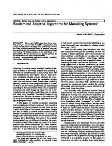
Figure 2.10 BER vs. delay spread for a 64-subcarrier OFDM system with different guard time.

Figure 2.11 shows the BER versus OFDM systems with different number of subcarriers N. Three multipath channels with delay spread of 2, 4, and 6 µ s are studied. No guard time is inserted to OFDM symbols. Simulation results show that in all cases, BER decreases as the number of subcarriers increases. For the same signal bandwidth, increasing the number of subcarriers increases the symbol duration. The ratio of the number of distorted samples to the total number of samples per OFDM symbol decreases as the symbol duration increases and thus the BER is decreased.

22


10

0

max. delay spread=2us max. delay spread=4us max. delay spread=6us 10

-2

BER

10

-1

10

10

10

-3

-4

-5

5

5.5

6

6.5

7

7.5

8

8.5

9

9.5

10

log2 N Figure 2.11 BER vs. number of subcarriers in a 5-multipath environment with delay spread exceeds guard time.

As mentioned in section 2.9, channel coding helps to recover symbols on the subcarriers that are located in the deep nulls of a frequency-selective channel. Figure 2.12 shows the amplitude response of a multipath channel having several deep nulls across the channel bandwidth. The multipath channel consists of two equal-power components, with the second component arriving four symbol periods later. Figure 2.13 shows the BER versus Eb /No for two 64-subcarrier OFDM systems operating in this channel, one without coding and the other one with (64,32) ReedSolomon coding. The guard time is longer than the delay spread to avoid ISI. Simulation results show that the OFDM system with RS coding has much better BER performance compared with the one without coding at high Eb N o .

23


2 1

Amplitude (dB)

0 -1 -2 -3 -4 -5 -6

0

10

20


50

60

Figure 2.12 Amplitude response of a two-ray multipath channel with the second multipath component arrived at four-symbol period later. 10

-1

uncoded coded

BER

10

10

10

10

-2

-3

-4

-5

6

7

8

9

10 11 fd (Hz)

12

13

14

Figure 2.13 BER vs. Eb /No in a two -ray channel with delay spread less than guard time.

24

15


2.10.2

BER Performance in Time-varying Multipath Environment

This section provides the performance evaluation of OFDM systems in the time-varying multipath environment. Figure 2.14 shows the BER versus Doppler frequency f d in a 5-multipath environment. Three OFDM systems with number of subcarriers 256, 512 and 1024 are studied. In all cases, guard time is longer than the delay spread so that no ISI is introduced by the channel. The figure shows that the BER performance for the 1024-subcarrier OFDM system is the worst among all three systems for all Doppler frequencies. The reason is that its long symbol duration decreases the frequency spacing between subcarriers and thus the frequency offset caused by the Doppler shift gives high level of ICI to the 1024-subcarrier OFDM system.

10

BER

10

10

10

-1

-2

-3

-4

N=256 N=512 N=1024 10

-5

50

100

150

200

250

300

f (Hz) d

Figure 2.14 BER vs. Doppler frequency in a 5-multipath channel with delay spread less than guard time.

Figure 2.15 shows the same scenario as the previous one but without guard time for OFDM symbols. As a result, symbols are corrupted by both ICI and ISI. For OFDM systems with N=64 and N=128, since the symbol duration is short, the ratio of distorted samples due to ISI to the total number of samples per OFDM symbol is large compared with the OFDM systems with N=512 and N=1024. Therefore, OFDM systems with small number of subcarriers have high BER even for the low Doppler frequency case. For the 512-subcarrier and 1024-subcarrier OFDM systems,

25

CHAPTER 2: INTRODUCTION TO OFDM the BER is lower than other OFDM systems for the low Doppler frequency case because their symbols have long duration to combat ISI and ICI is not high enough to cause significant degradation. However, as the Doppler frequency increases, the effect of ICI for those two systems is more significant than other OFDM systems and the BER increases as a result. The 1024-subcarrier OFDM system has higher BER than the 256-subcarrier OFDM and the 128subcarrier OFDM system when fd is higher than 100 Hz and 200 Hz respectively. Its BER exceeds the 64-subcarrier OFDM system when fd is higher than 300 Hz.

BER

10

10

-1

-2

N=64 N=128 N=256 N=512 N=1024 10

-3

50

100

150

200

250

300

f (Hz) d

Figure 2.15 BER vs. Doppler frequency in a 5-multipath channel with no guard time.

2.11 Chapter Summary In this chapter, we introduced the basic concept of OFDM, including ISI, ICI, guard time, and one-tap equalizers. We also studied the effect of the number of subcarriers and the guard time duration on the performance of OFDM systems. Furthermore, we explained the relationships between various OFDM parameters and also compared the difference between OFDM and single carrier communication systems. Finally, we presented simulation results for an OFDM system with various parameter values in both static and time-varying multipath environment.

26

Chapter 3 : Fundamentals of Adaptive Antenna Arrays

A transmitted signal is distorted when it travels through a non-ideal channel. A non-ideal channel is the one that does not have constant amplitude and linear phase response [31]. A filter is implemented at the receiver to extract information from this distorted signal. For example, a time-dispersive channel is a non-ideal channel which stretches a transmitted signal in time and causes ISI. A temporal filter, also known as a time-domain equalizer, is used to compensate the time-dispersive nature of the channel [31]. Time-dispersion implies frequency-selective fading and thus a frequency-domain equalizer can be used as the counterpart of the time-domain equalizer to compensate the frequency-selective nature of the channel [25]. On the other hand, a spatial filter collects a set of data over a spatial aperture using an antenna array and combines them based on a certain criterion to separate the desired signal from the interfering signals having the same frequency content but originating from different spatial locations. This process is known as beamforming [6]. An antenna array consists of a set of antenna elements that are spatially distributed at known locations with reference to a common fixed point [32]. The three most common geometries of antenna elements are linear, circular, and planar. A linear array consists of a set of antenna elements that are aligned along a straight line, while for a circular array antenna elements are distributed along a circle. On the other hand, a set of antennas located on a plane forms a planar array. A circular array is a special form of planar array in which the antennas are located on a horizontal plane in a circular fashion. A uniformly spaced linear array, whose antenna elements are spaced equally along a straight line, is the focus of this research.

3.1

Uniformly Spaced Linear Array

Figure 3.1 shows a uniformly spaced linear array with K identical isotropic elements, with the rightmost element as the reference element.

27

CHAPTER 3: FUNDAMENTALS OF ADAPTIVE ANTENNA ARRAYS

Array normal Plane wave

θ

Incident plane wave

d sin θ

Reference element d K

3

d 2

1

Figure 3.1 A uniformly spaced linear antenna array.

We assume that a single source transmits from a far distance so that the received signal at the antenna array is considered to be a plane wave incident at an angle θ with respect to the array normal. According to Figure 3.1, the plane wave first reaches the first antenna element, which is the reference element, and propagates all the way to the K-th antenna element. The bandpass representation of the received signal at the first antenna element can be expressed as x%1 (t ) = Re[ x1 ()exp{ t j 2π f ct}] ,

(3.1)

where x1 (t ) is the complex envelope representation of the received signal and f c is the carrier frequency. The propagation delay from the first to second antenna element is τ=

d sin θ , c

(3.2)

where c is the speed of the light. Therefore, the received signal at the second antenna element with respect to the received signal at the first antenna can be expressed as x% 2 (t ) = Re[ x1 (t − τ )exp{− j 2π f c (t − τ )}] ,

(3.3)

If the carrier frequency is large compared with the bandwidth of the signal, the narrowband signal model can be applied here, in which a small time delay can be modeled as a simple phase shift. In this case, equation 3.3 can be rewritten as

28

CHAPTER 3: FUNDAMENTALS OF ADAPTIVE ANTENNA ARRAYS x% 2 (t ) = Re[ x1 exp{− j 2π f c (t − τ )}] ,

(3.4)

and its complex envelope representation is given by x 2 (t ) = x1 ()exp( t − j 2π f cτ ) .

(3.5)

Substitute equation 3.2 into 3.5, we have d sin θ   x2 (t ) = x1 (t) exp  − j 2π fc  c    2π  = x1 (t) exp − j d sin θ  , λ  

(3.6)

where λ is the wavelength of the carrier. Since the antenna elements are uniformly distributed across the antenna array, the propagation delay along any two consecutive elements is the same and therefore the complex envelope representation of the received signal at the k-th antenna element can be expressed as  2π  xk (t ) = x1 (t) e x p − j (k − 1)d sin θ  , k = 1,K, K . λ  

(3.7)

We could also express the received signal in terms of vector notation. Define x (t ) = [ x1 ( t), x2 (t ),..., xK (t )]T , a (θ ) = [1, e

−j

2π d sin θ λ

,..., e

−j

(3.8)

2π (K −1) d sin θ T λ

] ,

(3.9)

the complex envelope representation of the received signal can be expressed as x (t ) = a (θ )x1 (t ) ,

(3.10)

where a (θ ) is known as the array response vector or the steering vector. Note that if the reference element is the leftmost element instead of the rightmost element, equation 3.10 will be written as a (θ ) = [1, e

j

2π d sinθ λ

,..., e

j

2π (K −1) d sin θ T λ

] .

(3.11)

If we assume that we have multiple users transmitting at the same time, and assume that all antenna elements are isotropic and the channel is AWGN, we can express the complex envelope representation of the received signal as follows:

29

CHAPTER 3: FUNDAMENTALS OF ADAPTIVE ANTENNA ARRAYS U

x (t ) = ∑ a (θ i ) si (t ) + n(t ) ,

(3.12)

i =1

where U is the number of users, θ i is the angle of arrival (AOA) for the i-th user, si (t ) is the transmitted signal for the i-th user, n (t ) denotes the K x 1 vector of the noise at the array elements, and a (θ i ) = [1, e

−j

2π d sinθ i λ

,..., e

−j

2π (K − 1)d sinθ i T λ

]

(3.13)

is the array response vector for the i-th user. In matrix notation, equation 3.12 becomes x (t ) = A(θ) s( t ) + n(t ) ,

(3.14)

A (θ ) = [a (θ1 ),a (θ 2 ),..., a (θ U )]

(3.15)

where

is the K x U matrix of the array response vectors and s(t ) = [ s1 ( t), s2 (),..., t sU (t )]T .

(3.16)

Furthermore, if there are multiple users transmitting at the same time at the same frequency in a multipath environment, and all the multipath components for a particular user arrive within the symbol duration, x (t ) can be expressed as U

Li

x (t ) = ∑∑α l ,i a (θ l ,i )si( t ) + n(t ) i =1 l =1 U

= ∑ bi si (t ) + n (t ) ,

(3.17)

i =1

where Li is the number of multipaths for the i-th user, α l ,i is the complex amplitude of the l-th multipath component for the i-th user, θl , i is the AOA of the l-th multipath component for the i-th user, a (θ l ,i ) is the array response vector corresponding to θl , i , and bi is the spatial signature for the i-th user and is defined as Li

b i = ∑α l ,i a(θ l ,i ) .

(3.18)

l =1

We can express equation 3.17 in the matrix form as x (t ) = Bs(t ) + n(t ) ,

30

(3.19)

CHAPTER 3: FUNDAMENTALS OF ADAPTIVE ANTENNA ARRAYS where B = [b1, b 2 ,..., bU ]

(3.20)

is the K x U spatial signature matrix with columns associated with the spatial signature of each transmitted signal. Suppose that we sample the received signal x (t ) M times at t1 ,t 2 ,...,t M , equation 3.14 can be expressed as X = A(θ )S + N ,

(3.21)

where X and N are the K x M matrices X = [x (t1 ), x (t2 ),..., x(t M )]

(3.22)

N = [ n(t1 ), n (t2 ),..., n(t M )]

(3.23)

S = [s (t1 ), s (t 2 ),..., s(t M )] .

(3.24)

and S is the U x M signal matrix

The array response vector in equation 3.9 represents the case in which each antenna element is isotropic. The term “isotropic” means that each antenna element can radiate or receive energy uniformly in all directions. In practice, antenna elements usually have non-uniform radiation patterns. One needs to perform array calibration to determine the array response vector for a range of angles and carrier frequencies. This can be done by placing a transmitter at various spatial locations and transmitting signals with different frequencies to estimate the array response vector of the antenna array. For a group of antenna elements that have similar but non-isotropic radiation pattern, the array beam pattern can be calculated based on the principle of pattern multiplication [33] as: G(θ ) = f (θ )F (θ ) ,

(3.25)

where f (θ ) is the radiation pattern for a set of antenna elements that have similar radiation pattern and F (θ ) is the array factor which is defined as F (θ ) = V T a(θ ) ,

(3.26)

V = [V1 ,V2 ,...,VK ]T

(3.27)

where

31

CHAPTER 3: FUNDAMENTALS OF ADAPTIVE ANTENNA ARRAYS is the weight vector with each element Vi corresponding to the k-th antenna element gain and a (θ ) is the array response vector defined in equation 3.9.

3.2

Beamforming

As mentioned earlier, the objective of beamforming is to separate the desired signal from interfering signals, given that they have the same frequencies but different spatial locations. Interfering signals can be the delayed version of the desired signal originated from the multipath environment or signals generated by other users. A digital beamformer samples the propagated wave field at the input of each antenna element, weights them based on a certain performance criterion and then combines them at the output of the beamformer. There are two types of beamformers, one for narrowband signals and one for wideband signals. Figure 3.2 shows a narrowband beamformer. A narrowband signal sampled at the k-th antenna element at time n is just the phase-shifted version of the signal received at the reference antenna element at time n. Since this phase shift is a function of the distance between the first antenna element and the k-th antenna element, a narrowband beamformer needs to sample the propagating wave field in space only. The signal at the output of the beamformer at time n, y(n), is given by a linear combination of the data at the K sensors at time n: K

y ( n) = ∑ wk xk ( n) , ∗

(3.28)

k =1

where * represents the complex conjugate, x k (n ) is the complex envelope representation of the received signal from the k-th antenna element at time n, and wk is the complex weight applied to x k (n ) . Equation 3.28 can be represented in vector form as

y ( n) = w H x( n) ,

(3.29)

where H denotes the Hermitian (complex conjugate) transpose and

w = [ w1 , w2 ,..., wK ]T

(3.30)

is the complex weight vector. Each sensor is assumed to have any necessary receiver electronics and an A/D converter if beamforming is performed digitally.

32


x1 (n)

W1*

x2 (n)

W2*

∑

xK (n )

y (n)

WK*

Figure 3.2 A narrowband beamformer.

Figure 3.3 shows a wideband beamformer. A wideband signal sampled at the k-th antenna element at time n is not just only a phase shift but also time delayed with respect to the signal received at the reference antenna element sampled at time n. This requires a wideband beamformer to sample the propagating wave field in both space and time. The output of a wideband beamformer can be expressed as K M −1

y (n ) = ∑ ∑ w*k ,m x k ( n − m) ,

(3.31)

k =1 m =0

where M-1 is the number of delays in each of the M sensor channels. Equation 3.31 can also be expressed in vector form as in equation 3.29, where w = [ w1,0 ,..., w1, M −1, ,..., wK ,0 ,..., wK ,M −1 ]T

(3.32)

and x (n ) = [ x1 (n ),..., x1 (n − M + 1),..., xk (n ),..., xk ( n − M + 1)]T .

In this case, both w and x( n) are KM x 1 column vectors.

33

(3.33)


x1 (n)

Z-1 * W1,1

* W1,0

x2 (n)

* WK,1

W1,*M -1

Z-1

Z-1 * W2,1

* W2,0

xK (n )

Z-1

W2,* M -1

Z-1

∑

y (n)

Z-1 * WK,2

WK,* M -1

Figure 3.3 A wideband beamformer.

The wideband beamformer shown in Figure 3.3 is more complex than the narrowband beamformer shown in Figure 3.2. To reduce the complexity, a wideband beamformer can be implemented in the frequency domain, as illustrated in Figure 3.4. As shown in equation 3.7, the signal received at the k-th antenna element has a phase shift of (2π / λ )(k − 1)d sin θ with respect to the signal received at the reference antenna element. For wideband signals, the frequency components at the two edges of the band may be widely different. Since λ = c / f , their

34

CHAPTER 3: FUNDAMENTALS OF ADAPTIVE ANTENNA ARRAYS corresponding wavelengths can be widely different and thus the phase shifts experienced by the frequency components at the two edges of the band are not equal. Therefore, it is intuitive that a wideband signal can be decomposed into frequency components and data at each frequency component is processed by their own beamformers. A frequency-domain beamformer first accumulates the sampled signal in buffer memories (not shown in Figure 3.4) at each antenna element to form N-point data blocks. It then takes an Npoint DFT of the data at each antenna element using the FFT algorithm and performs beamforming on individual frequency bins to accommodate different phase shifts experienced by each of them. At the output of the beamformer, an N-point IDFT is performed to convert the data back to the time domain. The output of the beamformer at frequency r, Y(r), is given by a linear combination of the data at the K sensors at frequency r: K

Y (r ) = ∑ Wk*,r X k (r ) ,

(3.34)

k =1

where Wk , r is the weight at r-th frequency bin at the k-th antenna element, and X k ( r) is the r-th bin DFT of x ( n) from the k-th antenna element. In vector form, equation 3.34 can be written as Y( r) = WrH X( r) ,

(3.35)

Wr = [W1,r ,W2,r ,...,WK , r ]T

(3.36)

X( r) = [X 1 ( r), X 2 (r ),..., X K (r)]T .

(3.37)

where

and

By proper selection of beamformer weights and careful data partitioning, the frequency domain beamformer output is equivalent to the wideband beamformer output.

35


X 1 ( R − 1) N-point DFT

X 1 (1) X 1 (0)

W1,*R-1 * W1,1

* W1,0

X 2 ( R − 1) N-point DFT

X 2 (1) X 2 (0)

W2,*R -1

Y ( R − 1)

* W2,1

Y (1)

* W2,0

N-point IDFT

Y (0)

∑

X K ( R − 1) N-point DFT

X K (1) X K (0)

W1,*R-1 * WK,1

* WK,0

Figure 3.4 A frequency-domain beamformer.

3.3

Spatial Filtering and Spatial Nyquist Sampling Theorem

As mentioned at the beginning of the chapter, a spatial filter can be considered as the counterpart of a temporal filter to extract the desired signal from interfering signals, with one operating in the spatial domain and the other one in the time domain. This can be shown by comparing the harmonic retrieval problem using a temporal filter with the beamforming problem using a spatial filter [34].

36

CHAPTER 3: FUNDAMENTALS OF ADAPTIVE ANTENNA ARRAYS A temporal filter is implemented by a tapped-delay-line filter. We consider a problem of using a tapped-delay-line filter to extract a sinusoid of certain frequency from a sinusoid composed of q frequency components. The input of the tapped-delay-line filter is expressed as q

x(t ) = ∑ ak exp{ j (2π f k t + φk )} + n (t ) ,

(3.38)

k =1

where f k , a k , and φ k are the frequency, amplitude, and phase, respectively, of the k-th sinusoid. Suppose we sample the input at every Ts sampling period unrelated to the frequency of the unknown sinusoid, and let x(i) denote the signal at time instant iTs , the sampled input signal can be written as q

x(i) = ∑ ak exp{ j (2π f k (iTs ) + φk )} + n (iTs ) .

(3.39)

k =1

After passing the signal to the tapped-delay-line filter with P-1 delay elements, the filter input and the P-1 outputs of the delay elements at the i-th sampling instant can be expressed as q

x (i) = ∑ a( f k ) sk (i) + n (i) ,

(3.40)

k =1

where x (i ) = [ x( i), x(i − 1),..., x(i − P + 1)]T , n (i ) = [ n(iTs ),..., n ((i − P + 1)Ts )]T , a ( fk ) = [1, e− j 2π f kTs ,..., e− j 2 π f k ( P−1) Ts ]T ,

(3.41)

and sk (i) is the k-th complex sinusoid at the i-th sampling instant defined as sk (i) = ak exp{ j (2π f k (iTs ) + φk )} .

(3.42)

Comparing equation 3.40 and 3.41 with the narrowband beamforming problem of equation 3.12 and 3.13, the following correspondences can be observed [6]: •

The normalized element spacing d / λ of the spatial filter corresponds to the sampling period Ts of the temporal filter, and

•

The sine of the AOA θ i , sinθ , of the spatial filter corresponds to the temporal frequency f k of the temporal filter input.

According to the Nyquist sampling theorem [8], in order to avoid aliasing, the sampling frequency of the temporal filter must be at least twice the highest frequency of the input signal. Since there is a correspondence between the temporal filter and the spatial filter, a corresponding theorem, named spatial Nyquist sampling theorem, is applied to the spatial filter. In the spatial

37

CHAPTER 3: FUNDAMENTALS OF ADAPTIVE ANTENNA ARRAYS domain, since λ / d corresponds to the sampling frequency of the temporal filter, and the highest frequency corresponds to 1 (since the largest value for sinθ is 1), the spatial Nyquist sampling theorem states that λ ≥ 2 ×1 , d

(3.43)

or equivalently, d≤

λ . 2

(3.44)

That is, the spacing between two antenna elements should be less than or equal to a half wavelength of the input signal in order to avoid aliasing. Spatial aliasing corresponds to an ambiguity in source locations. This means that the array response vectors for two different angles are the same, i.e., a (θ 1 ) = a (θ 2 ) , where θ 1 ≠ θ 2 .

(3.45)

Even though the antenna spacing satisfies the spatial Nyquist sampling theorem, equation 3.45 can still happen when θ 2 = π − θ1 since sin θ = sin(π − θ ) . This type of ambiguity is referred to as array ambiguity. Array ambiguity happens in the uniformly spaced linear array but not in the non-linear spacing array such as the circular array. Antenna spacing larger than a half wavelength causes aliasing; on the other hand, small antenna spacing not only reduces spatial discrimination because of the ill-dispersed of the array response vectors in the N dimensional vector space but also causes mutual coupling effects [35]. In practice, the antenna spacing is often kept near a half wavelength so that the spatial aliasing is avoided and the mutual coupling effect is minimized.

3.4

Criteria for Optimal Weights

An adaptive beamformer is able to adjust the weight on each antenna element based on the statistics of the array data. In general, it adjusts the weight vector such that it places nulls in the direction of interfering signals in an attempt to maximize the SNR at the beamformer output. Since the statistics of the array data may not be known and may change over time, adaptive algorithms are typically employed to determine the weights.

Most adaptive beamforming

algorithms involve iterative process to adjust the weights until a certain performance criterion is

38

CHAPTER 3: FUNDAMENTALS OF ADAPTIVE ANTENNA ARRAYS met. The most common performance criteria are the minimum mean-squared error (MMSE), maximum signal-to-interference-plus-noise ratio (MSINR) and linearly constrained minimum variance (LCMV). This section describes some of the performance criteria for beamforming.

3.4.1

Minimum Mean-Squared Error

The objective of the MMSE criterion is to minimize the mean-squared error between the received signal y(n) and the desired signal d(n). Mathematically, the cost function to be minimized is J = E[ d( n ) − y(n ) ] , 2

(3.46)

where E[⋅] denotes the ensemble average operator. Substitute equation 3.29 into equation 3.46, we have J = E[ d( n ) − y(n ) ] 2

= E[{d ( n ) − y( n)}{d ( n ) − y (n)}∗ ] = E[{d ( n ) − w H x (n )}{d ( n ) − w H x(n )}∗ ] = E[ d( n ) − w H x (n )d (n )* − d (n )x H (n )w + w H x (n )x H ( n )w ] 2

= E[ d( n) ] − E[w H x (n) d( n) * ]− E[ d( n )x H (n )w] + E[w H x (n )x H (n )w ] 2

= E[ d( n) ] − w H p − p H w + w H Rw , 2

(3.47)

where R = E[x( n) x H (n )]

(3.48)

is the K x K correlation matrix of the array sensor inputs x(n) and p = E[ x(n )d * (n )] .

(3.49)

is the K x 1 cross-correlation vector between the array sensor inputs x(n) and the desired signal d(n). In order to minimize the cost function, we take the gradient of the cost function with respect to w and set it to zero: ∇ J = −2p + 2 Rw = 0 .

(3.50)

w opt = R −1p ,

(3.51)

Solving equation 3.50, we have

39

CHAPTER 3: FUNDAMENTALS OF ADAPTIVE ANTENNA ARRAYS which is referred to as the Wiener-Hopf equation or the optimum Wiener solution [33]. Equation 3.51 shows that in order to obtain the optimum weight vectors, we need the knowledge of two statistics: 1. The correlation matrix R of the array input vector x(n), and 2. The cross-correlation vector p between the array input vector x(n) and the desired signal d(n). If we express the correlation matrix R as R = R ss + R uu ,

(3.52)

where R ss = E[d 2 (n )]a (θ )a H (θ ) , R uu = E[u (n )u (n )H ] , and u (n ) is the K x 1 vector of the sum of all interfering signals sampled at the array sensor input, and apply the matrix inversion lemma [36] to R −1 , we have   −1 1 R −1 =   Ruu . 2 H −1 1 + E[d ( n)]a (θ )R uu a (θ ) 

(3.53)

Furthermore, if we assume high SNR, x (n ) ≈ d (n )a (θ ) and p = E[ d( n) a(θ ) d * (n )] = E[ d 2 (n )]a (θ ) ,

(3.54)

then the Wiener solution can be expressed as follows:   −1 E[d 2 (n)] w opt =   R uu a (θ ) 2 H −1 1 + E[d ( n)]a (θ )R uu a(θ )  −1 = β MMSE Ruu a(θ )

3.4.2

(3.55) (3.56)

Maximum Signal-to-Interference-plus-Noise Ratio

In this performance criterion, the weights can be chosen to directly maximize the output signalto-interference-plus noise ratio (SINR) [33]. If we define s(n ) as the K x 1 vector of the desired signal sampled at the array sensor input, the output signal power of the beamformer can be expressed as

40

CHAPTER 3: FUNDAMENTALS OF ADAPTIVE ANTENNA ARRAYS 2

σ s2 = E[ wH s(n ) ]

= E[{wH s(n )}{w H s(n )}* ] = w H s( n) s (n )H w = w H R ss w ,

(3.57)

where R ss = E[s (n )s (n )H ] is the K x K correlation matrix of the array sensor input for the desired user. Similarly, the output interference-plus-noise power can be written as 2

σ u2 = E[ w H u (n ) ]

= w H Ruu w ,

(3.58)

where R uu = E[u (n )u (n )H ] is K x K correlation matrix of the array sensor input for the interferers. The output SINR, (SINR)o is given by (SINR)o = =

σ s2 σ u2 w H R ssw H . w H Ruu w H

(3.59)

To maximize the output SINR, we take the derivative of equation 3.59 with respect to w and set it to zero, which gives the following result: R ss w =

w H R ssw R uu w w H Ruu w

= λ R uu w

(3.60)

Equation 3.60 appears to be a joint eigenvalue problem. The optimum weight vector is obtained by finding the largest eigenvalue λmax of the symmetric matrix R −uu1 R ss , i.e. R −uu1R ss w opt = λmax w opt .

(3.61)

and the maximum output SINR, (SINR)o ,max is defined by (SINR)o ,max =

H H wopt Rss w opt H H wopt R uu w opt

41

.

(3.62)

CHAPTER 3: FUNDAMENTALS OF ADAPTIVE ANTENNA ARRAYS Since R ss = E[d 2 (n )]a (θ )a H (θ ) , the optimum weight vector can be expressed in terms of the Wiener solution as follows: −1 w opt = β MSINR R uu a (θ )

(3.63)

where β MSINR =

E[d 2 (n )] H a (θ )w opt . λmax

(3.64)

Furthermore, if the interference is white, Ruu = σ 2 I , where σ 2 is the variance of white noise and I is the identity matrix. In this case, the weights can be chosen to directly maximize the output signal-to-noise ratio (SNR) [36]. The output noise power is defined by σ n2 = σ 2 wH w ,

(3.65)

and the output SNR is given by ( SNR)o = =

σ s2 σ n2 w H R ssw . σ 2w H w

(3.66)

Again, we take the derivative of equation 3.66 with respect to w and set it to zero to find the maximum SNR. Assuming σ 2 = 1 and subject to the constraint wH w = 1 , we obtain R ss w = λ w ,

(3.67)

which is again an eigenvalue problem. Similar to the case of MSINR, the optimum weight vector is obtained by calculating the largest eigenvalue λmax of R ss , i.e. R ss wopt = λmax wopt

(3.68)

and the maximum output SNR is defined by ( SNR) o,max =

42

λmax . σ2

(3.69)


3.5

Adaptive Algorithms for Beamforming

The previous section describes some of the performance criteria for calculating the optimum weight vector. In order to obtain the optimum weight vector, one needs to know the second-order statistics.

Since these statistics are usually unknown and change over time, adaptive

beamforming algorithms are employed to estimate them and update the weight vector over time. As the weights are iteratively adjusted, the performance of beamformer is closer to the desired criterion. The algorithm is said to be converged when such a performance criterion is met. This section describes some of the adaptive beamforming algorithms.

3.5.1

Least-Mean-Square Algorithm

The optimum Wiener solution given in equation 3.51 requires the calculation of the inverse of the correlation matrix R and this results in a high computational complexity. The Least-MeanSquare (LMS) Algorithm [36] avoids matrix inverse operation by using the instantaneous gradient vector ∇J (n ) to update the weight vector, i.e. w (n + 1) = w (n) +

1 µ [−∇J (n )] , 2

(3.70)

where µ is the convergence factor which controls the speed of convergence and its value is usually between 0 and 1. The LMS algorithm is based on the steepest-descent method [36] which recursively computes and updates the weight.

It is intuitively reasonable that successive

corrections to the weight vector in the direction of the negative of the gradient vector should eventually lead to the MMSE, at which point the weight vector assumes its optimum value. An exact measurement of the instantaneous gradient vector is not possible since this would require a prior knowledge of both the correlation matrix R and the cross-correlation vector p. Instead, an instantaneous estimate of the gradient vector ∇ˆ J (n ) is used, which is given by ˆ J (n ) = −2pˆ (n ) + 2 R ˆ (n )w( n) , ∇

(3.71)

ˆ (n ) = x (n) x H (n ) R

(3.72)

pˆ (n) = x( n) d * (n )

(3.73)

where

43

CHAPTER 3: FUNDAMENTALS OF ADAPTIVE ANTENNA ARRAYS are the instantaneous estimates of R and p defined in equatio n 3.48 and 3.49 respectively. Substituting equation 3.71, 3.72 and 3.73 into equation 3.70, we have ˆ (n) w w ˆ (n + 1) = w ˆ (n ) + µ [pˆ (n ) − R ˆ ( n )]

=w ˆ (n ) + µ x( n)[ d* (n ) − x H ( n )w ˆ ( n )] =w ˆ (n ) + µ x(n )e*( n) ,

(3.74)

which is the LMS algorithm. The LMS algorithm is a member of stochastic gradient algorithms since the instantaneous estimate of the gradient vector is a random vector that depends on the input vector x( n) . The LMS algorithm requires only 2M complex multiplications per iteration, where M is the number of weights used in the adaptive array [6]. The rate of convergence is slow for a small value of µ but this gives a good estimation of the gradient vector since a large amount of data is taken into account. On the other hand, a large value of µ makes the rate of convergence fast but gives a degraded estimation of the gradient vector since only a small amount of data is considered. Moreover, the rate of convergence may also depend on the eigenvalue spread χ (R) , which is defined by χ (R ) =

λmax , λmin

(3.75)

where λmax is the largest eigenvalue of R and λmin is the smallest eigenvalue of R. For white inputs, the eigenvalue spread χ (R) is equal to one and it does not have any effect on the rate of convergence. However, for the non-white inputs with large χ (R) , the rate of convergence takes on a directional nature. More details about the directionality of convergence are discussed in [36].

3.5.2

Sample Matrix Inversion Algorithm

The idea of sample matrix inversion (SMI) algorithm [37] is to estimate the correlation matrix R and the cross-correlation vector p based on the samples of the array sensor input in an observation interval, i.e., ˆ = R

N2

∑ x(n )x

H

( n)

n = N1

44

(3.76)


pˆ =

N2

∑d

*

( n )x ( n ) ,

(3.77)

n = N1

where N1 and N2 are the lower and upper limits of the observation interval, respectively. The weight vector is then calculated using the optimum Wiener solution: ˆ −1pˆ , w ˆ =R

(3.78)

which are then applied to the samples of array sensor input that are received within the same observation interval. In order to allow the array to adapt as the signal environment changes, the ˆ and the cross-correlation sample vector pˆ are re-estimated for each correlation sample matrix R

observation interval. Data that are outside the current observation interval do not have any effect on the calculation of the weight vector for the current observation interval. ˆ , the matrix inversion lemma can be To avoid matrix inversion of the correlation matrix R

applied, which is given by H ˆ −1 ˆ −1 ˆ −1 ( n ) = R ˆ −1 ( n − 1) − R ( n − 1) x ( n ) x ( n ) R ( n − 1) , R ˆ −1 ( n − 1) x ( n ) 1 + xH ( n) R

ˆ − 1 ( 0 ) = 1 I, ε > 0 . R ε

N1 ≤ n ≤ N 2

(3.79)

ˆ should be As a rule of thumb, the number of samples required to obtain the correlation matrix R

at least twice the number of antenna elements [38]. The rate of convergence for SMI is faster than that of LMS because it does not depend on the eigenvalue spread χ (R) , signal powers, arrival angles, and other parameters. The SMI algorithm using matrix inversion lemma requires 3.5M 2 +M complex multiplications per iteration, where M is the number of weights used in the adaptive array.

3.5.3

Recursive Least-Squares Algorithm

Unlike SMI which uses an observation interval to estimate both R and p, recursive least-squares (RLS) algorithm [36] uses the weighted sum to estimate them: n

Rˆ (n ) = ∑ λ n −i x (i) x H (i) i =1

45

(3.80)

CHAPTER 3: FUNDAMENTALS OF ADAPTIVE ANTENNA ARRAYS n

pˆ (n) = ∑ λ n −i d * (i )x( i ) ,

(3.81)

i =1

where 0 < λ ≤ 1 is the weighting factor or forgetting factor which determines how quickly the previous data are de-emphasized, and n is the observation interval 1 ≤ i ≤ n . Factoring out the terms corresponding to i = n in both equation 3.80 and 3.81, we have the following recursion for ˆ (n ) and pˆ (n ) : updating both R ˆ (n ) = λ R ˆ ( n − 1) + x( n) x H (n ) R

(3.82)

pˆ (n) = λpˆ (n − 1) + d * ( n) x(n ) .

(3.83)

Since it is the inverse of covariance matrix that is required to estimate the weight, we obtain the ˆ (n ) using the matrix inverse lemma: following recursive equation for the inverse of R ˆ −1 (n ) = λ −1 [R ˆ −1( n − 1) − q (n )x H (n )R ˆ −1( n − 1)] , R

(3.84)

where q (n) =

ˆ −1 (n − 1)x (n ) λ −1R ˆ −1 ( n− 1)x ( n) 1 + λ −1 x H (n )R

(3.85)

is the gain vector. By rearranging equation 3.85, we have ˆ −1 (n − 1) u(n ) − λ −1q (n )x H (n )R ˆ −1 ( n− 1)u( n) q (n) = λ −1R ˆ −1 (n − 1) − λ −1q( n) x H (n )R ˆ −1( n − 1)]u (n ) . = [λ −1R

(3.86)

We see from equation 3.84 that the expression inside the brackets on the right-hand side of ˆ −1 (n ) . Thus, substituting equation 3.84 into equation 3.86, we have equation 3.86 equals R q (n ) = Rˆ −1 (n)x ( n) .

(3.87)

Equation 3.87 shows that the gain vector q (n ) is defined as the array sensor input x( n) ˆ (n ) . transformed by the inverse of the correlation matrix R

Substituting equation 3.83 and 3.84 to the optimum Wiener solution in equation 3.51, the weight vector can be updated as follows: wˆ (n ) =Rˆ −1 (n )pˆ (n )

46

CHAPTER 3: FUNDAMENTALS OF ADAPTIVE ANTENNA ARRAYS ˆ −1( n − 1) − q( n) x H (n )R ˆ −1( n − 1)][λ pˆ (n − 1) + d * (n )x (n )] = λ −1[R ˆ −1 ( n − 1) p ˆ −1( n− 1)pˆ ( n − 1) ˆ (n − 1) − q(n )x H (n )R =R ˆ −1( n− 1)x( n) − λ −1d * ( n)q( n) x H (n )R ˆ −1( n− 1)x( n) + λ − 1 d * (n )R ˆ −1 ( n − 1) p ˆ −1( n− 1)pˆ ( n − 1) ˆ (n − 1) − q(n )x H (n )R =R ˆ −1( n − 1) − q (n )x H ( n)R ˆ −1( n − 1)]}x( n) + d * (n ){λ −1[ R ˆ −1 ( n − 1) p ˆ −1( n− 1)pˆ ( n − 1) ˆ (n − 1) − q(n )x H (n )R =R ˆ −1 ( n) x(n ) + d * (n )R ˆ −1 (n) x( n) . =w ˆ (n − 1) − q( n)x H (n )w ˆ (n − 1) + d * (n )R

(3.88)

Finally, using the fact that q (n ) = Rˆ −1 (n)x ( n) as in equation 3.87, we can update the weight vector as follows: w ˆ (n ) = w ˆ ( n − 1) + q (n )[ d * (n )− x H (n )w ˆ (n − 1)] =w ˆ (n − 1) + q (n )ξ * (n ) ,

(3.89)

where ξ (n ) is the a prior estimation error defined by ξ ( n) = d (n ) − x T (n )w ˆ * (n − 1) = d (n ) − w ˆ H ( n − 1)x(n ) .

(3.90)

Equation 3.90 shows that the estimated desired signal w ˆ H ( n − 1) x(n ) is based on the previous least-squares estimate of the weight vector that was made at time n − 1 .

The fundamental difference between the RLS algorithm and the LMS algorithm is that the convergence factor µ in the LMS algorithm is replaced by the inverse of the correlation matrix ˆ −1 (n ) . The resulting rate of convergence is typically an order of magnitude faster than the LMS R

algorithm. However, the computational complexity of the RLS algorithm is much higher than that of the LMS algorithm. It requires 4 M 2 + 4 M + 2 complex multiplications per iterations, where M is the number of weights used in the adaptive array [6].

47


3.6

Chapter Summary

In this chapter, we presented an overview of the antenna array and provided a mathematical analysis of the signal at the output of the antenna array. We explained several beamformer structures and the correspondence between an antenna array and a tapped-delay-line filter. We also introduced several beamforming criteria and described several adaptive algorithms which are used to adjust the weights so that the beamforming criteria are met under the changing environment.

48

Chapter 4 : Adaptive Beamforming for OFDM Systems

In this chapter, we propose a novel frequency-domain beamforming algorithm for OFDM systems to suppress interference in a multipath environment. The type of interference that we are interested is hostile and the goal of interferers is to destroy the integrity of the signal transmitted by the desired user to the intended receiver. This type of interfering signal is referred to as a jamming signal. Although there are many research activities in OFDM, only a few numbers of them involve in adaptive beamforming for OFDM systems.

Kim and Lee [45] proposed a time-domain

beamforming strategy for an OFDM system in an AWGN channel with the presence of other users. On the other hand, Li and Sollenberger [46] proposed the MMSE diversity combiner using the parameter estimator to suppress cochannel interference in a two-ray channel model. However, none of them considers the case of having interference power higher than the received power of the desired user. Moreover, none of them considers the performance of an adaptive antenna array for OFDM systems in the environment that is rich in multipaths, which is the main focus of this research.

4.1

Frequency-domain Beamforming

The m-th sample of an OFDM symbol at the output of an OFDM transmitter can be written as N −1  2π mn  xm = ∑ X n exp  j , 0 ≤ m ≤ N −1 , N   n =0

(4.1)

where N is the number of subcarriers and X n is the data symbol on the n-th subcarrier. We assume that each OFDM symbol is transmitted through a multipath channel with L discrete paths and the receiver deploys a uniformly spaced linear array consists of K elements. Using the narrowband model assumption, the m-th sample at the k-th antenna element can be written as L−1 2π   rm, k = ∑ hm, l xm exp − j ( ( k − 1) d sin θ )  + n m, k , 0 ≤ m ≤ N − 1 , λ   l =0

49

(4.2)

CHAPTER 4: ADAPTIVE BEAMFORMING FOR OFDM SYSTEMS where d is the antenna spacing, λ is the wavelength of the carrier, θ is the AOA with respect to the array normal, hm ,l is the complex random variable for the l-th path of the channel impulse response at time m, and nm, k is the AWGN at the k-th antenna element at time m. If we let ω k (θ ) be the phase shift of the received signal at the k-th antenna element with respect to the

received signal at the reference antenna element, equation 4.2 can be written as L−1

rm, k = ∑ hm, l x m exp {− jω k (θ )} + nm, k , 0 ≤ m ≤ N − 1,

(4.3)

l= 0

where ω k (θ ) =

2π (k − 1)d sin θ . λ

(4.4)

We assume that the guard time is longer than the delay spread so that ISI can be completely eliminated. The demodulated symbol on the n-th subcarrier at the output of FFT at the k-th antenna element can be written as [39] N −1 L −1   2π ml  Yn ,k = ∑ ∑ X m Hl ( n − m )exp  − j  +ω k (θ )   + N n, k m =0 l =0    N

 L−1   2π nl   = ∑ Hl (0)exp − j  + ω k (θ )   X n     N  l =0 +

N −1

L−1

∑ ∑X

m = 0,m≠ n l = 0

m

  2π ml  Hl ( n − m )exp  −j  +ωk (θ )  + N n ,k    N

= α n, k X n + β n , k + N n, k , 0 ≤ n ≤ N − 1 ,

(4.5)

where N n, k is the AWGN on the n-th subcarrier at the k-th antenna element, α n, k is the multiplicative distortion caused by the channel at the desired subcarrier at the k-th antenna element, β n ,k is the ICI term, and H l ( n − m) is the FFT of a time-variant mulipath channel hm ,l , which is defined as follows: Hl ( n − m) =

1 N −1  2π k (n − m )  ∑ hm, l exp − j N  . N k =0

(4.6)

If we assume the multipath channel is time-invariant over one OFDM symbol duration, H l ( n − m) in equation 4.6 becomes zero and thus there is no ICI and β n ,k = 0 in equation 4.5.

The multiplicative distortion α n, k in equation 4.5 can be eliminated by using a one-tap equalizer

50

CHAPTER 4: ADAPTIVE BEAMFORMING FOR OFDM SYSTEMS at the n-th subcarrier. However, α n, k contains ω k (θ ) , which provides the AOA information for beamforming. Thus equalization should not be performed in order to keep the AOA information. Instead, we leave the multiplicative distortion with the demodulated symbol and pass it to the beamformer so that it can steer the beam towards the direction of the desired user. Using the MMSE criterion, the beamformer should be able to minimize the effect of α n, k when the adaptive beamforming algorithm converges. Since the multiplicative distortion may be fairly distinctive across the subcarriers, a single beamformer with one set of weight vector will not be able to suppress the distortion across them effectively. Therefore, symbols on individual subcarriers should be processed by their own beamformers. In this way, each beamformer has its own set of weight vector which combines the demodulated symbols on its corresponding subcarrier in an optimal way. Figure 4.1 shows the structure of the OFDM receiver using the frequency-domain beamforming approach. After the FFT operation on each antenna element, demodulated symbols on each subcarrier are passed to the corresponding beamformers. The output of the n-th beamformer can be written as K

Pn = ∑ Wn*,k Yn ,k , 0 ≤ n ≤ N −1 ,

(4.7)

k =1

where Wn ,k is the weight on the k-th antenna element for the n-th beamformer and Yn ,k is the demodulated symbol on the n-subcarrier at the k-th antenna element defined in equation 4.5. Parallel-to-serial conversion is performed at the output of beamformers followed by symbol demodulation and decoding. Furthermore, the frequency-domain beamforming using the MMSE criterion allows an OFDM receiver to bypass equalization, since the weight vector of individual beamformers will attempt to minimize the effect of the multiplicative distortion associated with the demodulated symbols on individual subcarriers. This gives a big advantage because one needs to estimate the channel frequency response in order to perform equalization, and in the interference environment where the interference power is higher than the power of the desired signal, it is difficult to estimate the channel frequency response for the desired user. Thus, the frequency-domain beamforming scheme avoids the channel estimation problem under the interference environment. Having individual beamformers to process its own subcarriers is also an advantage for suppressing the narrowband interference. Narrowband interference corrupts only a portion of the

51

CHAPTER 4: ADAPTIVE BEAMFORMING FOR OFDM SYSTEMS signal bandwidth. Having multiple beamformers across the signal bandwidth provides flexibility so that individual beamformers are able to adjust their own weights to adapt different interference patterns that may be experienced by different subcarriers simultaneously.

YN −1,1

Antenna 1

RF to baseband conversion

rm ,1

FFT

* WN-1,1

Y1,1 Y0,1

* W1,1

* W0,1

YN −1,2

Antenna 2


rm ,2

FFT

Y1 , 2 Y0 , 2

PN −1

* W1,2

∑

* 0,2

W

P1

Parallel to Serial

P0

∑

YN −1, K

Antenna K


rm , K

FFT

Y1,K Y0, K

* W1,K

* W0,K

Figure 4.1 The structure of an OFDM receiver using the frequency-domain beamforming approach.

4.2

Adaptive Beamforming Algorithm Used in Simulation

In this research, the adaptive beamforming algorithm that we use is the RLS algorithm. As mentioned earlier, the frequency-domain beamforming processes the data on the subcarrier basis. Thus weights on each subcarrier should be updated across time, not frequency.

If the

convergence of an adaptive beamforming algorithm is slow, which is typical for the case of LMS

52

CHAPTER 4: ADAPTIVE BEAMFORMING FOR OFDM SYSTEMS algorithm, then the bit error rate will be high for an OFDM system with large number of subcarriers. Although the SMI algorithm has fast convergence rate, it would introduce large latency here, due to the requirement of collecting large number of data symbols in order to have enough statistics to estimate the correlation matrix for individual beamformers. Therefore the RLS algorithm is chosen over the LMS algorithm and the SMI algorithm for our studies.

4.3

Performance in Two-ray Channel

The number of subcarriers processed by each beamformer may increase depending on the frequency-selectivity of the channel. If the channel frequency response is relatively flat across several subcarriers, it is possible for each beamformer to process data across several subcarriers that have similar channel frequency response. However, as the channel frequency response across them starts to vary, the effectiveness of each beamformer to minimize the impact of the multiplicative distortion on data symbols across multiple subcarriers decreases. As an illustration of the performance limitation of a single beamformer on the number of subcarriers under the frequency-selective environment, we consider two two-ray multipath channels. Figure 4.2 shows the channel impulse response of these two multipath channels. Both channels have the same amplitudes of multipath components but different delay spread. Figure 4.3 shows the corresponding sampled channel frequency response observed by a 128-subcarrier OFDM system. We assume that the channel frequency response is flat from the each subcarrier perspective. Figure 4.3 shows that the frequency-selectivity of the channel increases as the delay spread increases.

∑

0.8944

fk

2

=1

T: one symbol duration

0.8944

∑

k

fk

2

=1

k

0.4472

0.4472 0

T

T

(a)

0 T (b)

Figure 4.2 Channel impulse responses of the two 2-ray channels

53

T

CHAPTER 4: ADAPTIVE BEAMFORMING FOR OFDM SYSTEMS

1 1

0.8 0.6

0

Phase (radian)

Amplitude (dB)

0.4 -1

-2

-3

0.2

(a)

0 -0.2 -0.4 -0.6

-4 -0.8 -5

20

40


100

-1

120

20

40


100

120

1 1

0.8 0.6

0

Phase (radian)

Amplitude (dB)

0.4 -1

-2

-3

0.2

(b)

0 -0.2 -0.4 -0.6

-4 -0.8 -5

20

40


100

120

-1

20

40


100

120

Figure 4.3 Channel frequency responses for the 2-ray channels shown in Figure 4.2a and b, respectively

A number of signal constellation diagrams are provided to give one the insight of effectiveness of using beamformers for suppressing the multiplicative distortion associated with demodulated symbols. Figure 4.4 and 4.5 show a number of 16QAM signal constellation diagrams for a 128subcarrier OFDM system with the two-ray channels shown in Figure 4.2a and Figure 4.2b respectively. In all these cases, we assume that the guard time is greater than the delay spread to avoid ISI and no AWGN is present.

Furthermore, we insert pilot symbols across all the

subcarriers and the RLS algorithm has converged before the decoding process begins. Using one frequency-domain beamformer per subcarrier, the multiplicative distortion associated with each demodulated symbols is largely suppressed for both channels. This shows that the performance of the frequency-domain beamforming is independent of the delay spread of the channel when each beamformer processes data symbols on one subcarrier only. Using one frequency-domain beamformer for two subcarriers, the distortion may still be acceptable for the channel shown in Figure 4.2a but may not be acceptable for the channel shown

54

CHAPTER 4: ADAPTIVE BEAMFORMING FOR OFDM SYSTEMS in Figure 4.2b when the AWGN is present. Finally, using one frequency-domain beamformer for four subcarriers are probably not acceptable for both two-ray channels due to large distortion shown on the signal constellation diagrams.

The channel variation across four adjacent

subcarriers is too much that using one set of weight vector is unable to minimize the effect of the multiplicative distortion on four symbols at the same time. As a result, the number of beamformers required for this frequency-domain beamforming scheme depends on how frequency selective a channel is. For a given bandwidth of an OFDM signal, the bandwidth of each subcarrier decreases as the number of subcarriers increases and the channel frequency responses become very similar across several adjacent subcarriers. In this case, it is possible to apply a single beamformer for a number of symbols on the neighboring subcarriers to reduce computational complexity. In general, one needs to make the tradeoff between the computational complexity and the BER performance.

55


4

4

4

3

3

3

2

2

2

1

1

1

0

0

0

-1

-1

-1

-2

-2

-2

-3

-3

-3

-4 -4

-4 -4

-3

-2

-1

0

1

2

3

4

-3

-2

-1

(a)

0

1

2

3

4

-4 -4

-3

-2

-1

(b)

0

1

2

3

4

1

2

3

4

(c)

Figure 4.4 16QAM signal constellation diagrams for a 128-subcarrier OFDM system with the channel shown in Figure 4.2a. (a) one beamformer for one subcarrier; (b) one beamformer for two subcarriers; (c) one beamformer for four subcarriers.

4

4

4

3

3

3

2

2

2

1

1

1

0

0

0

-1

-1

-1

-2

-2

-2

-3

-3

-3

-4 -4

-4 -4

-3

-2

-1

0

1

2

3

4

-3

-2

-1

(a)

0

(b)

1

2

3

4

-4 -4

-3

-2

-1

0

(c)

Figure 4.5 16QAM signal constellation diagrams for a 128-subcarrier OFDM system with the channel shown in Figure 4.2b. (a) one beamformer for one subcarrier; (b) one beamformer for two subcarriers; (c) one beamformer for four subcarriers.

56


4.4

Beampattern

To observe the interference suppression capability for the frequency-domain beamforming scheme, we will observe the beampattern for a number of beamformers at different subcarriers under the interference environment, which consists of 7 wideband jammers with jamming power 6 dB higher than the received power of the desired signal. Table 4.1 shows the spatial locations of the seven jammers with respect to the array normal.

Table 4.1 Spatial locations of seven wideband jammers. Interferer # 1 2 3 4 5 6 7

Spatial locations -900 -750 -500 -250 250 500 750

The desired user is located at 00 with respect to the array normal. An eight element uniform linear array (ULA) is assumed to be deployed at the receiver side. Figure 4.6 shows the beampatterns of 8 out of 512 beamformers for a 512-subcarrier OFDM system under the AWGN channel at Eb /No = 20 dB. The 8 beamformers are located at the 64-th, 128-th, 192-th, 256-th, 320-th, 384-th, 448-th, and 512-th subcarriers. It shows that all eight beamformers steer the beam towards the direction of the desired user and at the same time place null towards the direction of the jammers. The desired signals at all eight subcarriers have at least 26 dB gain over all the jamming signals and many of them have more than 30 dB gain over the jamming signals. This shows that our frequency-domain beamforming scheme is very effective for suppressing the jamming signals which have higher power than the desired signal.

57


-5 -10

-15

-15

-20 -25

-30 -35

-40

-20 0 20 Angle (degrees)

40

60

80

-40 -100

100

0 -5

-10

-10

-15

-15

Amplitude (dB)

0

-20 -25

-35

-35

-60

-40


40

60

80

-40 -100

100

0

0

-5

-5

-10

-10

-15

-15

-20 -25

-30 -35

-40

-40

-40


40

60

80

-45 -100

100

0

0

-5

-5

-10

-10

-15

-15

-20 -25

-30 -35

-60

-40


40

60

80

100

60

80

100

(d)

-80

-60

-40


40

60

80

100

(f)

-80

-60

-40


40

60

80

100

(h)

-25

-35

-80

40

-20

-30

-40 -100


-25

-35

-60

-40

-20

-30

-80

-60

-25 -30

-80

-80

-20

-30

Amplitude (dB)

Amplitude (dB) Amplitude (dB) Amplitude (dB)

-60

-5

-45 -100

(g)

-25

-35

-80

(b)

-20

-30

-40 -100

(e)

Amplitude (dB)

-5 -10

-40 -100

(c)

0

Amplitude (dB)

(a)

Amplitude (dB)

0

-40 -100

-80

-60

-40


40

60

80

100

Figure 4.6 Beampatterns for the beamformers at the (a) 64-th subcarrier, (b) 128-th subcarrier, (c) 192-th subcarrier, (d) 256-th subcarrier, (e) 320-th subcarrier, (f) 384-th subcarrier, (g) 448-th subcarrier, and (h) 512-th subcarrier. The circle indicates the location of desired user and the asterisk indicates the location of jammers.

58


4.5

System Parameters

The format of OFDM symbols generated at the transmitter side is the same as the ones we used for simulation in Chapter 2. We assume the source generates a bit stream at a rate of 20 Mbps. Using the 16QAM modulation scheme, the bandwidth of the OFDM signal is 5 MHz. We define a transmitted frame which consists of 100 OFDM symbols. In order to facilitate the convergence of the RLS algorithm, we send the first 12 symbols as the training symbols, leaving 88 symbols as the data symbols in a frame. The RLS algorithm uses the training symbols as the desired symbols to facilitate the convergence of the algorithm at the beginning of the frame. It then switches to the decision-directed mode during the data portion of the frame to update the weight vector for tracking the time-varying nature of the channel. During the decision-directed mode, the desired signal is the symbol at the output of the decision device. We set the forgetting factor of the RLS algorithm to 0.9999 in our simulation. We assume the receiver is equipped with an eight element ULA with half wavelength spacing between the elements. Each element of the antenna array is assumed to be isotropic. Figure 4.7 shows the simulation block diagram used for the evaluation of our proposed beamforming algorithm. Transmitter:

Data bits

16QAM modulation

Insert training symbols

IFFT

Add guard time

Flat/frequencyselective fading channel

Flat/frequencyselective fading channel

Wideband/narrowband Gaussian jammers

AWGN

Receiver:

Decoded bits

16QAM demodulation

Frequency-domain beamforming

FFT

Remove guard time

Figure 4.7 Simulation block diagram for an OFDM system using frequency-domain beamforming.

59


4.6

Simulation Results

In this section, we present the simulation results for the proposed beamforming algorithm for OFDM systems with the presence of interference. The following two cases will be studied: 1. Flat fading channel with two wideband/narrowband Gaussian jammers 2. Frequency-selective fading channel with two wideband Gaussian jammers. In both cases, we assume that the transmitter is located at a far distance and the received signal is considered as a plane wave. The objective of the first case is to illustrate the advantage of frequency-domain beamforming under the narrowband jamming environment while the objective of the second case is to show the interference suppression capability of the proposed scheme under a practical multipath channel model.

4.6.1

Flat Fading Channel

We would like to compare the performance of an OFDM system using one beamformer located at the center frequency bin to process all the symbols across subcarriers versus individual beamformers for each subcarrier under the flat fading channel. The Doppler frequency of the flat fading channel is assumed to be 10 Hz.

The fading is correlated within one frame but

independent for individual frames and also independent for each jamming signal. Two cases will be presented here, one is the wideband jamming case and the other one is the narrowband jamming case. Table 4.2 shows the spatial locations and the jamming power with respect to the power of the desired signal for the two cases. The desired user is located at 00 with respect to the array normal.

Table 4.2 Spatial locations and jamming power of two jammers with respect to the power of the desired signal in the flat fading channel in the simulation of the OFDM system. Case #

Type of interference

Locations 0

0

Jamming Power (dB)

1

Wideband

-40 , 40

13, 6

2

Narrowband (10% of the signal bandwidth)

-400 , 400

13, 6

Figure 4.8 shows the BER performance of a 512-subcarrier OFDM system for the wideband jamming case. The performance of an OFDM system using one beamformer is comparable to the one using 512 subcarriers. Since the channel is flat fading, the channel frequency response is the same across the subcarriers. Moreover, the wideband jammers corrupt the data symbols in the

60

CHAPTER 4: ADAPTIVE BEAMFORMING FOR OFDM SYSTEMS same manner across the subcarriers.

As a result, there is no need to employ individual

beamformers to suppress the multiplicative distortion and interference on the subcarrier-bysubcarrier basis.

10

0

num of beamformers=1 num of beamformers=512

-1

BER

10

10

10

-2

-3

0

2

4

6 Eb/No

8

10

12

Figure 4.8 BER vs. Eb /No for a 512-subcarrier OFDM system with two wideband jammers located at 400 and -400 in a flat fading channel

Figure 4.9 presents the BER performance of the same OFDM system for the narrowband jamming situation. Simulation result shows that an OFDM system using one beamformer per subcarrier has a better performance than the one using one beamformer for all the subcarriers. Since some subcarriers may be corrupted by the jamming sig nals coming from different directions while others may not receive any jamming signals at all, having one beamformer per subcarrier allows each beamformer to adjust its own weight vector so that optimum combining can be performed on each subcarrier based on the interference environment experienced by each of the subcarriers. Therefore, the BER is lower for the OFDM system using 512 beamformers than the one using one beamformer only.

61


10

0

num of beamformers=1 num of beamformers=512

-1

BER

10

10

10

-2

-3

0

2

4

6 Eb/No

8

10

12

Figure 4.9 BER vs. Eb /No for a 512-subcarrier OFDM system with two narrowband jammers located at 400 and -400 in a flat fading channel

4.6.2

Frequency-selective Fading Channel

In this section, we would like to apply our proposed beamforming algorithm under the frequencyselective fading environment and study its performance. The multipath channel model that we use is the COST-207 six-tap typical urban (TU) channel model, which is defined in Table 4.3 [40]. This channel model is often used to study the performance of dig ital video broadcasting (DVB) which uses OFDM as the modulation scheme.

Table 4.3 The COST-207 six-tap typical urban channel model. Tap number Delay ( µ s ) Frac. power

1 0.0 0.19

2 0.2 0.38

3 0.5 0.24

4 1.6 0.09

5 2.3 0.06

6 5.0 0.04

We assume that all six resolvable multipath components are within an angle spread of 300 with respect to the central arriving angle of the transmitted signal. Using the Jakes’ model [41], the complex amplitude of the l-th resolvable multipath component on the k-th antenna can be represented as [42]

62


hl , k (t ) =

Pl J

J −1

∑ exp{ j  2π f i =0

d

  2π  cos(Φl ,i )t + φl ,i  exp  j  d k sin(θ l ,i )  ,   λ

}

(4.8)

where Pl is the average power received for the l-th path (taken from the Table 4.3 for the simulation), J is the number of scatters composing each resolvable path, f d is the maximum Doppler frequency, φl , i is a uniformly distributed random phase, Φ l ,i is the random angle of departure relative to the motion of the mobile of each multipath, d k is the distance between antenna k and the reference antenna, λ is the carrier wavelength, and θ l ,i is the angle of arrival of each scattered replica with respect to the array normal. Moreover, we assume that θ l ,i is distributed as ∆l ∆l 1  , Θl − ≤ x ≤ Θl + 2 2 , pθl , i ( x ) =  ∆ l  0, otherwise 

(4.9)

where Θ l and ∆ l are the central angle of arrival and the angle spread of the l-th multipath, respectively. Table 4.4 shows the parameters used in equation 4.8 and 4.9 for our simulation.

Table 4.4 Parameters for the Jakes’ model J Φ ∆ φ

20 00 to 3600 50 0 0 to 3600

dk / λ fd

0.5k 10 Hz

We assume the channel is quasi-static, meaning that the channel is time-invariant over one OFDM symbol and thus no ICI is introduced to the system. We also assume that the delay spread of the channel is shorter than the guard time and thus ISI is eliminated completely. As mentioned before, the computational complexity of the frequency-domain beamforming scheme increases as the number of subcarriers increases. As stated in Chapter 3, the complex multiplications per iteration for the RLS algorithm is 4 M 2 + 4 M + 2 , where M is the number of weights used in the beamformer. For OFDM systems with N number of subcarriers, if we assign one beamformer to process data on one subcarrier only, the computational complexity for the frequency-domain beamforming algorithm is N (4 M 2 + 4 M + 2) . However, since the bandwidth

63

CHAPTER 4: ADAPTIVE BEAMFORMING FOR OFDM SYSTEMS per subcarrier is small for large number of subcarriers, the channel frequency responses across several neighboring subcarriers are similar and thus it may be possible to employ one beamformer to process several neighboring subcarriers.

Table 4.5 shows the number of complex

multiplications per iteration for an eight-element antenna array and the subcarrier bandwidth for an OFDM system with different number of subcarriers.

Table 4.5 Computational complexity of the RLS algorithm and bandwidth of each subcarrier for an OFDM system with different number of subcarriers. Number of subcarriers (N) 64 128 256 512 1024

Complex multiplications per iterations 18560 37120 74240 148480 296960

Bandwidth per subcarrier for 5MHz signal bandwidth (kHz) 78.125 39.063 19.531 9.766 4.883

We would like to study the performance degradation under the COST-207 TU channel model as the number of subcarriers processed by individual beamformers increases. We are interested in investigating the possibility of reducing the number of beamformers without significant degradation. We will use N=512 and N=1024 for our study because they are the ones that require high computational complexity. Since the bandwidth of OFDM signal remains the same, the duration of each frame for a 1024-subcarrier OFDM system is twice as long as the one with 512 subcarriers. As is conventional, we assume the channel is frequency non-selective from the perspective of each subcarrier. The desired user is transmitted at the spatial location of 00 with respect to the array normal. Three different cases are studied to investigate two wideband jammers at different locations. Table 4.6 shows the spatial locations and the received power of the two jammers with respect to the power of the desired signal for these three cases.

Table 4.6 Spatial locations and jamming power of two jammers with respect to the power of the desired signal in the frequency-selective fading channel in the simulation of the OFDM system. Case # 1 2 3

Locations -600 , 600 -400 , 400 -250 , 250

Jammer Power (dB) 13, 6 13, 6 13, 6

Figure 4.10, 4.11, and 4.12 show the BER versus Eb /No for a 512-subcarrier system for cases 1, 2, and 3. In each case, the total numbers of beamformers that are employed are 64, 128, 256, and

64

CHAPTER 4: ADAPTIVE BEAMFORMING FOR OFDM SYSTEMS 512. The performance of the OFDM system using one antenna element is also shown. For all three cases, simulation results show that an OFDM system using one antenna element is not able to suppress the jamming signals at all. For case 1 and 2, simulation results show that the BER performance for a 512-subcarrier OFDM system using 512 beamformers is very much the same as the one using 256 beamformers for low Eb /No with only a little improvement for high Eb /No . However, the performance degradation is noticeable for the case of 128 beamformers and is significant for the case of 64 beamformers. This comparable performance suggests that under this scenario one may use 256 beamformers for a 512-subcarrier OFDM system to reduce the computational complexity by half without significant degradation in performance. For case 3, the BER performance is worse than case 1 and 2 because for the 300 angle spread, the spatial range of the received jamming signals overlaps the spatial range of the received desired signal and thus the jamming signals may fall into the main beam of the desired user. In this case, an OFDM system using 128 beamformers has performance that is comparable to systems using 256 and 512 beamformers.

10

-1

BER

10

0

10

-2

num of beamformers=64 num of beamformers=128 num of beamformers=256 num of beamformers=512 1 antenna case 10

-3

0

2

4

6 Eb/No

8

10

12

Figure 4.10 BER vs. Eb /No for a 512-subcarrier OFDM system with two wideband jammers located at 600 and -600 in the COST 207 six-tap TU channel model.

65


10

-1

BER

10

0

10

-2


-3

0

2

4

6 Eb/No

8

10

12

Figure 4.11 BER vs. Eb /No for a 512-subcarrier OFDM system with two wideband jammers located at 400 and -400 in the COST 207 six-tap TU channel model. 10

-1

BER

10

0

10

-2


-3

0

2

4

6 Eb/No

8

10

12


66


Figure 4.13, 4.14, and 4.15 show the BER performance for the case of N=1024. The numbers of beamformers used for evaluation are 128, 256, 512, and 1024. For all 3 cases, simulation results show that there is not much improvement using 1024 beamformers rather than using 256 beamformers. However, the computational complexity can be reduced by a factor of four using 256 beamformers. This suggests that the channel is relatively flat across four subcarriers and therefore one beamformer is able to handling four neighboring subcarriers at the same time. Similar to the case of the 512-subcarrier OFDM system, there is significant performance degradation with two jammers located at -250 and 250 because some of the received jamming signals fall into the main beam of the desired user. The performance of the 1024-subcarrier OFDM system is worse than the 512-subcarrier OFDM system. The reason is because the symbol duration is double for the 1024-subcarrier OFDM system and the MSE between the desired signal and the received signal starts to increase towards the end of the frame. To improve the performance, one can insert some pilot symbols at the middle of the frame to maintain the MSE to the minimum level. However, the spectral efficiency decreases as a result. 10

-1

BER

10

0

10

-2


-3

0

2

4

6 Eb/No

8

10

12


67


10

-1

BER

10

0

10

-2


-3

0

2

4

6 Eb/No

8

10

12

Figure 4.14 BER vs. Eb /No for a 1024-subcarrier OFDM system with two wideband jammers located at 400 and -400 in the COST 207 six-tap TU channel model. 10

-1

BER

10

0

10

-2


-3

0

2

4

6 Eb/No

8

10

12


68


4.7

Chapter Summary

In this chapter, we proposed a novel beamforming algorithm for OFDM systems in the frequency-selective environment with the presence of interference.

We provided the

mathematical analysis of the frequency-domain beamforming scheme and proposed the adaptive algorithm that is used in this scheme. We also illustrated some beampatterns under the AWGN channel and analyzed its performance under the 2-ray channel model. Finally, we presented the simulation results of the proposed scheme for the 512-subcarrier and 1024-subcarrier OFDM systems using different number of beamformers under the flat fading and frequency-selective fading channels with the presence of interference.

69

Chapter 5 : Adaptive Beamforming for AV-OFDM Systems

In this chapter, we present the simulation model and simulation results for the AV-OFDM system employing an antenna array. The AV-OFDM system described here is a unique system proposed by the Raytheon Company. It uses OFDM as the choice of modulation. The main difference between a conventional OFDM system and the AV-OFDM system is that the AV-OFDM system is a spread spectrum system which uses Walsh orthogonal modulation to spread the signal to a bandwidth larger than the information bandwidth.

This provides low probability

interception/anti-jamming (LPI/AJ) capabilities for the signal.

5.1

AV-OFDM Waveform

Figure 5.1 shows the AV-OFDM signal space. The AV-OFDM waveform spans the twodimensional space: time and frequency. Direct sequence spread spectrum is employed to spread the signal in time while OFDM modulation is employed to allocate the spread signal across frequency. The whole signal bandwidth is partitioned into subbands whose bandwidth is limited to the coherence bandwidth.

As a result, the channel is frequency-nonselective from the

perspective of each subband. The spread spectrum signal, realized using Walsh orthogonal modulation, provides LPI/AJ capabilities while the subband partitioning provides resistance to multipath fading. Furthermore, a wide range of selection of the Walsh size and the number of subbands allow the AV-OFDM system to be adaptable to the changing environment.

70

CHAPTER 5: ADAPTIVE BEAMFORMING FOR AV-OFDM SYSTEMS

f1 f2 f3

f1024 FFT Block 1 frequency FFT Block 2

Walsh seq. 2

Walsh seq. 1

Walsh seq. M

f1 f2 f3 Subband 1

f1024 Subband 2

FFT Block N

Subband M

time

Figure 5.1 The AV-OFDM signal space.

5.2

AV-OFDM Transmitter

Figure 5.2 shows the baseband simulation block diagram for the AV-OFDM transmitter.

Bit stream RS Encoding

Walsh Modulation

Interleaving

real

complex

Zero padding and 2048-point IFFT

TRANSEC

Figure 5.2 Simulation block diagram for the AV-OFDM transmitter.

The bit stream is segmented into 6-bit symbols and the Reed-Solomon (RS) encoder is used to encode every K symbols into 64 coded RS symbols. The minimum Hamming distance for the RS (64,K) code is given by d min = 64 − K + 1 ,

and the number of errors t that can be corrected is given by

71

(5.1)

CHAPTER 5: ADAPTIVE BEAMFORMING FOR AV-OFDM SYSTEMS  64 − K  t= .  2 

(5.2)

After that, bits are modulated using the Walsh orthogonal modulation scheme. The Walsh orthogonal modulation maps every n bits into one of the 2 n Walsh functions according to the following formula: Walsh function number = 2 0 c0 + 2 1 c1 + 2 2 c2 + L + 2 n −1 cn −1 ,

(5.3)

where c0 represents the last coded bits and c n−1 represents the first coded bits. Each of the Walsh functions corresponds to a Walsh sequence with components in {+1, -1} generated using a Hadamard matrix. A Hadamard matrix of order 2 n is an 2 n x 2 n matrix of +1 and -1 components such that any pair of distinct rows or columns is orthogonal [26]. A Hadamard matrix H of order 2 n is generated as H n−1 H 2n =  2 H 2n−1

H 2n −1  , − H 2 n−1 

H1 = [1] .

(5.4)

All the row and column sequences of a Hadamard matrix are Walsh sequences. The Walsh function number generated in equation 5.3 is used as the row index of a Hadamard matrix to produce a Walsh sequence. The orthogonal property of a Walsh sequence can be mathematically represented as N

∑WAL i =1

m

N n = m , [i ]WALn [i] =  0 n ≠ m

(5.5)

where i is the chip index of the Walsh sequence and N is the size of the Walsh sequence. In our simulation, the size of Walsh sequence is either 32 or 1024. Walsh sequences are then placed into subbands sequentially. A subband consists of one or more subcarriers. An AV-OFDM system using 32-ary Walsh modulation consists of 1024 subbands with 1 subcarrier per subband while an AV-OFDM system using 1024-ary Walsh modulation consists of 128 subbands with 8 subcarriers per subband. The interleaver is able to place all the chips of a Walsh sequence on consecutive subcarriers or place them one by one for every several number of subcarriers based on the value of the interleaver depth. The interleaver processes the data slot-by-slot. Each slot contains 128 IFFT blocks. The value of the interleaver depth is a power of two. When the interleaver depth is 1, each Walsh sequence is sent by consecutive subbands for one IFFT block time. On the other

72

CHAPTER 5: ADAPTIVE BEAMFORMING FOR AV-OFDM SYSTEMS hand, when the interleaver depth is 128, each Walsh sequence is sent by one subband for 128 IFFT block time. Figure 5.3 and Figure 5.4 show the operation of the interleaver on one slot of Walsh sequences of size 1024 and 32 for several values of the interleaver depth respectively. Interleaver Depth = 1: Blk time 1 Subcarrier 1 Subcarrier 2

Subcarrier 1024

Blk time 128

Blk time 2

WAL2 [1]  WAL1[1]  WAL [2] WAL2 [2] 1   M M  WAL1[1024] WAL2[1024]

L L

WAL128 [1]  L L WAL128 [2]   O O M  L L WAL128[1024] 

Interleaver Depth = 2: Blk time 1

Blk time 128

Blk time 2

WAL 1[2]  WAL1 [1]  WAL [3] WAL1[4] Subcarrier 2  1  M M  WAL1[1023] WAL1[1024]  WAL2 [1] WAL2 [2]  WAL2 [4]  WAL2[3]  M M  Subcarrier 1024 WAL2 [1 023] WAL2 [1024] Subcarrier 1

L L L L

O O

L L L L L L

O O

L L

WAL127 [2]  WAL127 [3] WAL127 [4]   M M  WAL127 [1023] WAL127 [1024]  WAL128 [1] WAL128[2]   WAL128[3] WAL128[4]   M M  WAL128 [1023] WAL128[1024]  WAL127 [1]


Blk time 2

WAL1 [2]  WAL1[1]  WAL [5] WAL1 [6] 1 Subcarrier 2   M M  WAL1[1021] WAL1[1022]  M M  M M   WAL [1] WAL4[2] 4   WAL4 [5] WAL4[6]  M M  Subcarrier 1024 WAL4 [1021] WAL4 [1022] Subcarrier 1

Blk time 128

L L

O

WAL1[4] WAL1[8] M

L L L L

O O

WAL125[1]

WAL125[2]

WAL125[5]

WAL125[6]

M

M

L L

O

L WAL1[1024] L L WAL126[1021] WAL126 [1022] L L

M

L L

L

WAL4 [4]

L L

O

L

O

M

O O

WAL4 [8] M

L L

O O

M

M

M

M

WAL128[1]

WAL128[2]

WAL128[5]

WAL128[6]

M

M

L

O

L L

O

L WAL4 [1024] L L WAL128[1021] WAL128[1022] L

Figure 5.3 Interleaver operation for a slot of Walsh sequences of size 1024.

73

WAL125 [4]  WAL125[8]   M  WAL126 [1024]  M  M  WAL128 [4]   WAL128[8]   M  WAL128 [1024]

CHAPTER 5: ADAPTIVE BEAMFORMING FOR AV-OFDM SYSTEMS Interleaver Depth = 1: Blk time 1 Blk time 2

WAL9 [1]  WAL1[1]  WAL [1] WAL9 [2] 1   M M  WAL1[32] WAL9 [32]  M M  M M   WAL [1] WAL [1] 8 18   WAL8 [2] WAL18[2]  M M  Subcarrier 1024 WAL8[32] WAL18 [32] Subcarrier 1 Subcarrier 2

Blk time 128

L L L L

O O L

M

O O O O

L L L L

O O

L L

WAL1017[1]  WAL1017 [2]   M  WAL1017 [32]  M  M  WAL1024[1]   WAL1024 [2]   M  WAL1024 [32]


Blk time 2

Blk time 128

WAL1 [2]  WAL1 [1]  WAL [3] WAL1 [4] Subcarrier 2  1  M M  WAL [31] WAL 1 1[32]   M M  M M   WAL [1] WAL [2] 16 16   WAL16 [3] WAL16 [4]  M M   Subcarrier 1024 WAL16 [31] WAL16 [32] Subcarrier 1

L L L L

O O

L L

O O O O

L L L L

O O

L L

WAL1009 [2]  WAL1009 [3] WAL1009 [4]   M M  WAL1009[31] WAL1009 [32]  M M  M M  WAL1024[1] WAL1024 [2]   WAL1024 [3] WAL1024 [4]   M M  WAL1024 [31] WAL1024 [32] WAL1009[1]

Interleaver Depth=4: Blk time 1 Subcarrier 1 Subcarrier 2

Subcarrier 1024

Blk time 2

WAL1[2]  WAL1 [1]  WAL [5] WAL1[6] 1   M M   WAL1[29] WAL1[30]  M M  M M   WAL [1] WAL [2] 32 32   WAL32 [5] WAL32 [6]  M M  WAL32 [29] WAL32[30]

L L

O

Blk time 128

WAL1[4] WAL1[8] M

L WAL1[32] L

M

L

WAL32[4]

O

L

O

M WAL32 [8] M

L L L L

O O

WAL993 [1]

WAL993[2]

WAL993 [5]

WAL993[6]

M

L L WAL993[29]

O

M

L

L

WAL993[30] L

M

L L

WAL1024 [1]

WAL1024 [2]

WAL1024 [5]

WAL1024 [6]

L L

O O

M

M

L

M

L L O O

L

M

M

O

L

O

L WAL32[32] L L WAL1024 [29] WAL1024 [30] L

Figure 5.4 Interleaver operation for a slot of Walsh sequences of size 32.

74

WAL993[4]  WAL993 [8]   M  WAL993[32]   M  M  WAL1024 [4]   WAL1024[8]   M  WAL1024 [32]

CHAPTER 5: ADAPTIVE BEAMFORMING FOR AV-OFDM SYSTEMS Each data block of size 1024 at the output of the interleaver is then scrambled by a TRANSEC PN sequence. This provides protection against enemy exploitation of the known Walsh code sets. Since we do not have a true TRANSEC PN code, we generate a complex random code sequence of length 1024 with +1 and -1 values as the TRANSEC PN code and multiple it to the Walsh sequence for our simulation. After that, each sequence is twice-oversampled by inserting 1024 number of zeros in the middle of a data block. This oversampling process is necessary in order to reduce aliasing during the digital-to-analog (D/A) conversion process, although our baseband simulation is limited to the digital domain only. Inserting zeros at the middle of a data block corresponds to mapping onto frequencies close to positive and negative half the sampling rate while the data samples are modulated onto subcarriers around 0 Hz when IFFT is performed. Finally, an AV-OFDM symbol with 2048 samples is produced at the output of IFFT.

5.3

AV-OFDM Receiver

The AV-OFDM receiver is basically the reverse operation of the AV-OFDM transmitter. Figure 5.5 illustrates the baseband simulation block diagram for the AV-OFDM receiver.

2048-point FFT and data extraction

complex

real

Deinterleaving

Walsh Decoding

RS Decoding

DETRANSEC

Figure 5.5 Simulation block diagram for the AV-OFDM receiver.

Each received AV-OFDM symbol is first demodulated from subcarriers using the FFT operation. Then 1024 data samples are extracted by selecting the first 512 and last 512 samples from a block of 2048 FFT samples. Afterwards, each data block is descrambled by multiplying with the same TRANSEC PN sequence that is used on the transmitter side. Since we assume perfect chip synchronization, received Walsh sequences are produced when the two identical PN sequences are multiplied together. Deinterleaving is then performed to allocating Walsh sequences into subbands and Walsh decoding is performed to estimate the transmitted Walsh sequences. For the m-th received Walsh sequence, a Walsh decoder determines whic h of the N possible Walsh sequences was transmitted based on the highest correlation measure between the m-th received

75

CHAPTER 5: ADAPTIVE BEAMFORMING FOR AV-OFDM SYSTEMS sequence and all the N possible Walsh sequences. The correlation measure between the m-th Walsh sequence and the n-th Walsh sequence is defined as [43] N

WALm ,WALn = ∑ WALm [i ]WALn [i ] ,

(5.6)

i =1

and the Walsh decoder estimates the transmitted Walsh function number by carrying out the following operation: Estimated Walsh function number = max

n = 1,..., n= N

WALm , WALn .

(5.7)

Walsh function numbers are then converted to the corresponding bits by performing decimal-tobinary conversion. Finally, the RS decoder is used to decode the bits.

5.4

Adaptive Beamforming Algorithms

In our study, we simulate the AV-OFDM system using an antenna array and evaluate its performance under different jamming cases. The criteria that we employed for beamforming in the AV-OFDM system are the MSINR and MSNR. Recall in equation 3.63 of Chapter 3, the optimum weight vector obtained using the MSINR criterion consists of the correlation matrix of the interfering signal and the array response vector. The equation is reproduced here for convenient: −1 w opt = β MSINR R uu a (θ ) ,

(5.8)

where R −uu1 is the inverse of the correlation matrix of the interfering signal, a (θ ) is the array response vector, and β MSINR is a scalar whose value does not affect the performance of the MSINR beamformer. To apply this beamforming algorithm, we need to collect samples of interfering signals at the receiver before receiving the desired signal to estimate the correlation matrix R uu and also the AOA of the desired signal to calculate the weight vector. Moreover, since it is not practical to perform matrix inversion in real-time, the matrix inversion lemma that is employed in the SMI algorithm is used to estimate R −uu1 recursively. In our simulation, the time we spend on collecting the samples of interfering signal is equivalent to 10% of the duration of one data slot, which will be defined later in this chapter. Figure 5.6 shows the beamformer structure of the AV-OFDM system using the MSINR criterion.

76

The MSINR beamformer

CHAPTER 5: ADAPTIVE BEAMFORMING FOR AV-OFDM SYSTEMS combines the received Walsh sequences at the output of the de-interleaving before Walsh decoding.

2048-point FFT

Deinterleaving

DE-TRANSEC 2048-point FFT

Deinterleaving

∑

Walsh Decoding

RS Decoding

DE-TRANSEC

2048-point FFT

Deinterleaving

DE-TRANSEC

Figure 5.6 The receiver structure of the AV-OFDM system using the MSINR criterion.

In the environment where there are no scatters around the transmitter and receiver, optimum performance is achieved by steering the beam towards the direction of the desired signal while steering nulls towards the direction of interfering signals. However, when there are many scatters surrounding the receiver and there is no line of sight (LOS) between the transmitter and the receiver, the interfering signals arrive to the receiver at a wide range of angles and the interference becomes spatially white. In this case, MSNR criterion may be used to obtain the optimum weight vector. Using the MSNR criterion, the optimum weight vector is calculated by solving the following eigenvalue problem: R ss wopt = λmax wopt ,

77

(5.9)

CHAPTER 5: ADAPTIVE BEAMFORMING FOR AV-OFDM SYSTEMS where R ss is the correlation matrix of the desired signal and λmax is the largest eigenvalue of the correlation matrix R ss . The optimum weight vector is the eigenvector associated with the largest eigenvalue of the correlation matrix R ss .

In AV-OFDM, the adaptive beamforming algorithm using the MSNR criterion can be implemented by post-processing the signal at the output of the de-interleaver. We define the matrix of correlation measures between the m-th received Walsh sequences at the output of the Kelement antenna array and all possible Walsh sequences as

RWAL

 WAL1m ,WAL1   WAL2m ,WAL1   M = k  WALm ,WAL1  M  K  WAL ,WAL m 1 

WAL1m ,WAL2

L L

WAL2m ,WAL2

L L

M

O O

WAL ,WAL2

L L

M

O O

k m

K m

WAL ,WAL2

L L

WAL1m ,WAL N   WAL2m ,WAL N   M   , k WALm ,WAL N   M  K WALm ,WAL N 

(5.10)

where WALkm is the m-th received Walsh sequence at the k-th antenna element and N is the number of possible transmitted Walsh sequences. Then we pass the correlation measure matrix to the MSNR beamformer. The output of the beamformer can be represented as y = w H RWAL ,

(5.11)

y = [ y1 , y2 ,K , y N ]

(5.12)

where

is the 1 x N vector of the combined correlation measures and w is the MSNR weight vector. The estimated Walsh function number is the index of y where the maximum value is located, i.e. Estimated Walsh function number = index ( max {y}) .

(5.13)

The largest element of y corresponds to the largest eigenvalue of the correlation matrix R ss in equation 5.9. The MSNR weight vector is updated by selecting the column of the correlation measure matrix R WAL whose index is the same as the estimated Walsh function number.

We refer to this adaptive beamforming algorithm as the MSNR algorithm. In order to ensure that the badly corrupted received Walsh sequences are not used to update the MSNR weight vector, a

78

CHAPTER 5: ADAPTIVE BEAMFORMING FOR AV-OFDM SYSTEMS threshold is defined to verify the quality of a received Walsh sequence. In an interference-andnoise free environment, due to the orthogonal property of the Walsh functions, the correlation measure between the received Walsh sequence and the corresponding transmitted Walsh sequence is equal to the Walsh size while all the other correlation measures are zeros. Based on this observation, we can define a quality measure for each received Walsh sequence. Reordering the elements of y in equation 5.12 such that y = [ y i1 , y i2 ,K , yi N ], 1 ≤ in ≤ N , n = 1,2,L, N

(5.14)

with yi1 ≤ yi2 ≤ L ≤ yiN , we define a quality measure as κ =

yi N−1 yiN

.

(5.15)

Obviously, κ is between 0 and 1. The smaller the value of κ is, the better the quality of the received Walsh sequence is. In our research, we set the threshold of 0.85 and the MSNR weight vector is updated only if κ ≤ 0.85 . Figure 5.7 shows the beamformer structure of the AV-OFDM system using the MSNR criterion.

79


DE-TRANSEC

DE-TRANSEC

Deinterleaving

Measure Correlation

Measure Correlation

Measure Correlation

Deinterleaving

Deinterleaving

∑

Find the index of the largest element

RS Decoding

80

2048-point FFT

2048-point FFT

2048-point FFT

DE-TRANSEC

Figure 5.7 The receiver structure of the AV-OFDM system using the MSNR criterion.


5.5

Simulation Cases

We assume that the AV-OFDM receiver deploys a 4-element ULA with half wavelength spacing between the elements. Each element of the antenna array is assumed to be isotropic. The desired user is located at 300 with respect to the broadside of the array. Three types of jamming cases are studied: 1

Three Wideband Jammers Three wideband jammers generate white Gaussian noise.

Table 5.1 shows the spatial

locations with respect to the broadside of the antenna array and the interference power of the three wideband jammers with respect to the power of the desired signal for the case of 32-ary and 1024-ary Walsh modulation. 2

Single Strong Wideband Jammer One strong wideband Gaussian jammer is located at 600 with respect to the broadside of the array. The interference power is 20 dB and 30 dB gain with respect to the power of the desired signal for 32-ary Walsh modulation and 1024-ary Walsh modulation respectively.

3

Three Narrowband Jammers Three narrowband jammers generate Gaussian noise with bandwidth approximately 10% of the desired signal bandwidth. The spatial locations and the interference power of the three narrowband jammers are the same as the three wideband-jammer case shown in Table 5.1.

Table 5.1 Spatial locations and interference power of the three jammers with respect to the power of the desired signal in the simulation of the AV-OFDM system. 600 13 3

Location Power in dB (Walsh size = 1024) Power in dB (Walsh size = 32)

900 6 0

00 6 0

Two types of channels are investigated in our simulation for the above jamming cases. They are the flat fading channel and the static frequency-selective channel. For the flat fading cases, we assume Doppler frequency of 20 Hz and no angle spread for the received signal, resulting in completely correlated fading across the antenna array. The fading is correlated within one slot duration but independent for individual slots and also independent for each jamming signal. For the frequency-selective channel, we use the Elliptical channel model [44] to generate the multipath environment, which will be explained later in section 5.7.2.

81


5.6

System Parameters

The AV-OFDM waveform has a wide range of signal format parameters to choose from. Table 5.2 provides the values of parameters that are used for the simulation in our research.

Table 5.2 A V-OFDM signal parameters. Slot duration (preamble+data) Data burst Bandwidth M-ary Walsh modulation Number of subbands Number of subcarriers RS code rate

5.72 ms 5.12 ms 25.6 MHz 32,1024 1024 (for 32-ary), 128 (for 1024-ary) 1024 0.5

Based on the parameters specified above, the following parameters can be calculated as follows: •

The number of IFFT blocks for one slot is N IFFTblk =

•

data burst . NIFFTblk

(5.17)

Stream data rate is Rdata =

•

bandwidth ∗ number of bits per Walsh word . Walsh word size

(5.19)

Information bit rate is Rinfo =

•

(5.18)

Number of data bits per slot is Ninfo = R data * data burst * code rate .

•

(5.16)

Duration for one IFFT block is TIFFTblk =

•

Walsh size ∗ number of subbands . number of subcarriers

N info slot duration

.

(5.20)

Processing gain per data bit is  Walsh word size  PG = 10log  .  number of bits per Walsh word ∗ code rate 

82

(5.21)


Table 5.3 shows the values of the above parameters for our simulation based on the parameter values specified in Table 5.2.

Table 5.3 Parameter values for the 32-ary and 1024-ary Walsh modulation schemes. 32-ary Walsh modulation

1024-ary Walsh modulation

N IFFTblk

128

128

TIFFTblk

40 µ s

40 µ s

Rdata

138 Kbps

4 Mbps

Ninfo

353

10240

Rinfo

61.5 Kbps

1.79 Mbps

PG

23 dB

11 dB

The interleaver depth is different for the wideband and narrowband jamming cases and also for the flat fading and frequency-selective fading channels. For the flat fading channel, we set the interleaver depth of 1 for the wideband jamming case. Since the flat fading is highly correlated within a short period of time, setting the interleaver depth of 1 allows all the Walsh sequences to be sent sequentially in time with minimum loss of orthogonality among them. However, for the narrowband jamming situation, we set the interleaver depth of 32.

This can prevent the

possibility of corrupting the whole Walsh sequence for the case of 32-ary Walsh modulation, because the whole Walsh sequence is not allocated at consecutive subcarriers but at every 32 subcarriers. For the frequency-selective fading channel, the interleaver depth is set to 128 so that each Walsh sequence is sent within the bandwidth of one subband to minimize the effect of frequency-selective fading.

5.7

Simulation Results

This section provides the simulation results for the cases described in section 5.6. In order to study the performance degradation due to the error in estimating AOA, we have two versions of MSINR weight vectors. The first one has the perfect estimation of AOA and is named as SMI1 and the second one has 150 of AOA estimation error and is named as SMI2.

Both SMI

algorithms calculate the weight vector at the beginning of the slot and then apply it for the whole slot. For the MSNR algorithm, we use the SMI weights calculated at the beginning of the slot as the initial weights and update the weights for each Walsh sequence using the MSNR algorithm. Two versions of the MSNR algorithm are studied. The first one named MSNR1 uses the weight

83

CHAPTER 5: ADAPTIVE BEAMFORMING FOR AV-OFDM SYSTEMS vector calculated by SMI1 as the initial weight. The second version, named MSNR2, uses the weight calculated by SMI2 as the initial weight. Simulation results are presented into two categories: the flat fading channel and the frequency-selective fading channel.

5.7.1

Flat Fading Channel

Figure 5.8 shows the BER vs. Eb /No for the three-wideband-jammer case with 1024-ary Walsh modulation. The SMI1 algorithm has 2 dB gain over the SMI2 algorithm at the BER of 10-3 . For low Eb /No , the performance of the SMI algorithm due to the AOA estimation error can be improved by employing the MSNR algorithm. However, for high Eb /No , such improvement does not exist.

The reason is because for the case of low SNR, white noise is the dominant

interference after dispreading and thus the adaptive algorithm using the MSNR criterion can improve the performance over the SMI algorithm with AOA estimation error. However, for high SNR, the jamming signal is the dominant interference. Therefore, the adaptive algorithm using the MSINR criterion is more effective than the MSNR criterion. Figure 5.9 shows the BER for the three-wideband-jammer case with 32-ary Walsh modulation. Simulation result shows that performance is worse compared with the 1024-ary Walsh modulation. The reason is because of the low processing gain. The MSNR post-processing does not help to improve the performance for the SMI beamforming with 150 AOA estimation error even for low SNR. Figure 5.10 and 5.11 show the beampatterns of the SMI1 and MSNR1 algorithm for the 1024-ary Walsh modula tion at Eb /No = 10 dB. For the SMI1 algorithm, the desired user has a gain of approximately 11 dB over the strongest jammer among the three jammers. However, for the MSNR1 algorithm, the gain is reduced to 5 dB over the strongest jammer and thus the BER increases.

84


10

0

SMI1 SMI2 MSNR1 MSNR2

BER

10

10

10

10

-1

-2

-3

-4

0

2

4

6 Eb/No

8

10

12

Figure 5.8 BER vs. Eb /No for the three-wideband-jammer case with Walsh size of 1024 in a flat fading channel. 10

0


-1

BER

10

10

10

-2

-3

0

2

4

6 Eb/No

8

10

12

Figure 5.9 BER vs. Eb /No for the three-wideband-jammer case with Walsh size of 32 in a flat fading channel.

85


5

0

Amplitude (dB)

-5

-10

-15

-20

-25 -100

-80

-60

-40


40

60

80

100

Figure 5.10 Beampattern for the three-wideband-jammer case with Walsh size of 1024 using the SMI1 algorithm in a flat fading channel.

5

0

Amplitude (dB)

-5

-10

-15

-20

-25 -100

-80

-60

-40


40

60

80

100

Figure 5.11 Beampattern for the three-wideband-jammer case with Walsh size of 1024 using the MSNR1 algorithm in a flat fading channel.

86

CHAPTER 5: ADAPTIVE BEAMFORMING FOR AV-OFDM SYSTEMS Figure 5.12 and 5.13 present the case when there is a single strong wideband jammer for 1024-ary and 32-ary Walsh modulation respectively. For both cases, the jamming power is higher than the processing gain of the desired signal. Simulation result shows that the BER performance of the adaptive algorithm using the MSINR criterion for the strong wideband jammer case is similar to the three-wideband-jammer case for 1024-ary Walsh modulation and better for 32-ary Walsh modulation. However, the adaptive algorithm using the MSNR criterion cannot suppress the jammer and results in a devastating performance. Figure 5.14 and 5.15 show the beampatterns of the SMI1 and MSNR1 algorithms for the 1024ary Walsh modulation at Eb /No = 10 dB respectively. The SMI1 algorithm is very effective to suppress the strong interfering signal with 300 of spatial difference from the desired user. The desired signal has approximately 23 dB gain over the jamming signal. However, the MSNR1 algorithm gives an adverse effect by steering the beam towards the direction of the strong jammer and therefore its BER performance is disastrous.

87


10

BER

10

10

10

10

0

-1

-2

-3

SMI1 SMI2 MSNR1 MSNR2 -4

0

2

4

6 Eb/No

8

10

12

Figure 5.12 BER vs. Eb /No for the single strong-wideband-jammer case with Walsh size of 1024 in a flat fading channel. 10

BER

10

10

10

10

0

-1

-2

-3

SMI1 SMI2 MSNR1 MSNR2 -4

0

2

4

6 Eb/No

8

10

12

Figure 5.13 BER vs. Eb /No for the single strong-wideband-jammer case with Walsh size of 32 in a flat fading channel.

88


5

0

Amplitude (dB)

-5

-10

-15

-20

-25 -100

-80

-60

-40


40

60

80

100

Figure 5.14 Beampattern for the single strong-wideband-jammer case with Walsh size of 1024 using the SMI1 algorithm in a flat fading channel. 5

0

Amplitude (dB)

-5

-10

-15

-20

-25 -100

-80

-60

-40


40

60

80

100

Figure 5.15 Beampattern for the single strong-wideband-jammer case with Walsh size of 1024 using the MSNR1 algorithm in a flat fading channel.

89

CHAPTER 5: ADAPTIVE BEAMFORMING FOR AV-OFDM SYSTEMS Figure 5.16 and 5.17 show the BER result when there are three narrowband jammers and the Walsh sizes of the desired user are 1024 and 32 respectively. Simulation result shows that the performance is better compared with the case when the interference is wideband for high Eb /No . For 1024-ary Walsh modulation, the performance of the SMI1 algorithm is 0.8 dB better than the SMI2 algorithm at the BER of 10-3 . Similar to the three-wideband-jammer channel, the MSNR algorithm does not provide any improvement to the SMI beamforming with 150 AOA estimation error in most Eb /No cases. Figure 5.18 and 5.19 show the beampatterns of the SMI1 and MSNR1 algorithms for the 1024ary Walsh modulation at Eb /No = 10 dB respectively. For the SMI1 algorithm, the desired user has approximately 15 dB gain over the strongest jammer among the three jammers. However, for the MSNR1 algorithm, the desired user has only 4 dB gain over the jammer. In all three jamming cases, the beampattern plots show that the MSNR algorithm has the tendency to steer the beam towards the direction of the received signal with the strongest power.

90


10

0


BER

10

10

10

10

-1

-2

-3

-4

0

2

4

6 Eb/No

8

10

12

Figure 5.16 BER vs. Eb /No for the three-narrowband-jammer case with Walsh size of 1024 in a flat fading channel. 10

0


BER

10

10

10

10

-1

-2

-3

-4

0

2

4

6 Eb/No

8

10

12

Figure 5.17 BER vs. Eb /No for the three-narrowband-jammer case with Walsh size of 32 in a flat fading channel.

91


5

0

Amplitude (dB)

-5

-10

-15

-20

-25

-30 -100

-80

-60

-40


40

60

80

100

Figure 5.18 Beampattern for the three-narrowband-jammer case with Walsh size of 1024 using the SMI1 algorithm in a flat fading channel.

4 2 0

Amplitude (dB)

-2 -4 -6 -8 -10 -12 -14 -100

-80

-60

-40


40

60

80

100

Figure 5.19 Beampattern for the three-narrowband-jammer case with Walsh size of 1024 using the MSNR1 algorithm in a flat fading channel.

92


5.7.2

Frequency-selective Fading Channel

We use the Elliptical channel [44] model to generate the multipath environment and study the performance of the AV-OFDM system under frequency-selective fading. In this model, a large number of scatters are uniformly distributed within an ellipse. The transmitter and receiver are located at the two foci points of the ellipse. Figure 5.20 shows the concept of the Elliptical channel model Scatters

RX

TX

Elliptical Scattering Region Figure 5.20 The Elliptical channel model.

The size of the ellipse is completely described by its semi-major and semi-minor axis. The choice of these two parameters determines the maximum delay spread τ max of the channel, which in turn determines the strength of the multipath components. Signal which takes a long time to travel from a transmitter to a receiver has lower received power compared with the one traveling at a short time. The Elliptical channel model is suitable to model the urban environment where there are many scatters surrounding the transmitter and the receiver. Table 5.4 illustrates various parameters that are used to generate multipath components for our simulation. In our simulation, the locations of scatters change slot-by-slot.

Table 5.4 Parameters of the Elliptical channel model. Number of scatterers Maximum delay spread Doppler spread Angle spread Tx-Rx separation Path loss exponent

100 7.8 µ sec (200 chips) None [0 2π] 1 km 4

93

CHAPTER 5: ADAPTIVE BEAMFORMING FOR AV-OFDM SYSTEMS Since the elliptical channel has an angle spread of 3600 , there is no discrete AOA associated with the desired signal. Thus, we evaluate only the SMI1 algorithm and the MSNR1 algorithm. Furthermore, we study the wideband jamming case only. Figure 5.21 and 5.22 show the BER for the three-wideband-jammer case with 1024-ary and 32ary Walsh modulation respectively. Simulation result shows that the BER performance for the MSNR1 algorithm outperforms the SMI1 algorithm. The reason is because the SMI beamformer steers the beam towards the direction of the desired user but minimizes the gain in other directions. However, since the received signals could come from any directions due to multipath propagation, the receiver should not limit the antenna gain to the direction of the desired user. The MSNR post-processing adjusts the antenna gain to maximize the SNR and thus improves the BER performance. Figure 5.23 and 5.24 show the beampatterns of the SMI1 and MSNR1 algorithms for the 1024ary Walsh modulation at Eb /No = 10 dB respectively. The MSNR1 algorithm does not steer the beam towards any particular direction but collects the signals from all the directions in order to maximize the desired SNR.

94


10

0

SMI1 MSNR1

-1

BER

10

10

10

-2

-3

0

2

4

6 Eb/No

8

10

12

Figure 5.21 BER vs. Eb /No for the three-wideband-jammer case with Walsh size of 1024 in a frequencyselective fading channel.

10

0

SMI1 MSNR1

-1

BER

10

10

10

-2

-3

0

2

4

6 Eb/No

8

10

12

Figure 5.22 BER vs. Eb /No for the three-wideband-jammer case with Walsh size of 32 in a frequencyselective fading channel.

95


4 2 0

Amplitude (dB)

-2 -4 -6 -8 -10 -12 -14 -16 -100

-80

-60

-40


40

60

80

100

Figure 5.23 Beampattern for the three-wideband-jammer case with Walsh size of 1024 using the SMI1 algorithm in a frequency-selective fading channel. 4 2 0

Amplitude (dB)

-2 -4 -6 -8 -10 -12 -14 -16 -100

-80

-60

-40


40

60

80

100

Figure 5.24 Beampattern for the three-wideband-jammer case with Walsh size of 1024 using the MSNR1 algorithm in a frequency-selective fading channel.

96


5.8

Chapter Summary

In this chapter, we presented the AV-OFDM system. We introduced the AV-OFDM signal space and described its transmitter and receiver structures in detail. Then we proposed two adaptive beamforming algorithms using the MSINR and MSNR criteria for the AV-OFDM system. Finally, we provided simulation results for two different Walsh modulation schemes under the flat fading and frequency-selective fading with three types of jamming environment. In general, the MSINR algorithm has a better BER performance compared with the MSNR algorithm in the flat fading environment but not in the frequency-selective environment.

97

Chapter 6 : Conclusions and Future Work

6.1

Conclusions

In this thesis, we study the adaptive array algorithms for OFDM systems and AV-OFDM systems.

The nature of the multicarrier communication gives new challenges for applying

adaptive beamforming to OFDM. We propose a frequency-domain beamforming scheme for conventional OFDM systems which operate under a frequency-selective environment. The main idea behin d this scheme is to employ multiple beamformers, with each beamformer combining symbols for each subcarrier. Using the MMSE criterion, this scheme can minimize the effect of multipath distortion introduced by the frequency-selective channel without the loss of the AOA information. The proposed beamforming algorithm has been studied in both flat fading and frequency-selective fading channels with the presence of interference. Simulation results show that using individual beamformers to process data symbols on each subcarrier has a better performance than using one beamformer only under the narrowband jammer case in the flat fading channel. We also show that under the COST 207 six-tap TU channel model, the total number of beamformers can be fewer than the number of subcarriers for OFDM systems with 512 and 1024 subcarriers without significant performance degradation. For the AV-OFDM system, we propose two adaptive beamforming algorithms using the MSINR and MSNR criteria and evaluate these two algorithms under the flat and frequency-selective fading channels. Simulation results show that in general the BER performance is better using Walsh size of 1024 than using Walsh size of 32 due to larger processing gain. The MSINR beamforming using the SMI algorithm outperforms the MSNR algorithm in the flat fading channel but requires AOA estimation. The MSNR post-processing tends to steer the beam towards the direction of the strongest received signal. It has superior performance to the SMI algorithm under the frequencyselective environment, where the desired signal does not have a particular but a wide range of AOA to the receiver. At the beginning of this thesis, we also introduce a basis concept of OFDM and the fundamentals of adaptive antenna array.

98

CHAPTER 6: CONCLUSIONS AND FUTURE WORK

6.2

Future Work

The following lists some of the possible of future work on adaptive beamforming for OFDM systems. 1

In this thesis, we only evaluate the performance of the beamforming algorithms for the receiver employing ULA. It may be useful to study its performance for different array geometries, such as the circular array and the planar array.

2

In this research, we only employ the RLS algorithm for the frequency-domain beamforming scheme. After the RLS algorithm converges, it may be possible to use the LMS or the normalized LMS algorithm to reduce the computational complexity. The performance of the adaptive beamforming algorithm using the LMS algorithm in the decision-directed mode should be examined in the future.

3

In the simulation, we only apply the frequency-domain beamforming scheme to the outdoor channel model. Its performance should also be studied under the indoor channel model. In fact, the IEEE 802.11g standard, which is the standard for the next generation of WLANs in 2.4GHz and 5GHz radio band, supports OFDM as one of the modulation schemes. Furthermore, we can study the performance of this scheme under the IEEE 802.11 environment since this standard is primarily for indoor applications.

4

It would be interesting to apply the frequency-domain beamforming scheme to the AVOFDM system and study its performance for the frequency-selective environment. Since in an AV-OFDM system, the bandwidth of each subband is considered to be flat, each beamformer should be able to process data symbols across the subcarriers within one subband.

5

In this research, we assume no carrier frequency offset between the transmitter and receiver and also perfect symbol timing at the receiver.

In the future, we can examine the

performance of the beamforming algorithms under the frequency offset, phase noise, and symbol timing error conditions. 6

Last but not least, it will be useful to implement the proposed beamforming algorithms in a DSP or FPGA board and construct the 8-element antenna array for field trial testing.

99

REFERENCES

[1]

J. M. Pereira, “Balancing Public and Private in Fourth Generation,” The 12th IEEE International Symposium on Personal, Indoor and Mobile Radio Communications, vol. 2, pp 125-132, Sept/Oct 2001.

[2]

A. Bria, F. Gessler, O. Queseth, R. Stridh, M. Unbehaun, J. Wu, and J. Zander, “4th Generation Wireless Infrastructures: Scenarios and Research Challenges,” IEEE Personal Communications, vol. 8, issue: 6, pp. 25-31, December 2001.

[3]

P. Mahonen and G. C. Polyzos, “European R&D on Fourth-Generation Mobile and Wireless IP Networks [Guest Editorial],” IEEE Personal Communications, vol. 8, issue: 6, pp. 6-7, December 2001.

[4] R. Van Nee and R. Prasad, OFDM for Wireless Multimedia Communications, Artech House Publishers, Massachusetts, 2000. [5] J. H. Winters, J. Salz, and R. D. Gitlin, “The Impact of Antenna Diversity on the Capacity of Wireless Communication Systems,” IEEE Transactions on Communications, vol. 42, no. 2/3/4, February/March/April 1994. [6] B. Van Veen and K. Buckley, “Beamforming: A Versatile Approach to Spatial Filtering,” IEEE ASSP Magazine, pp. 4-22, April 1988. [7] M. Russell and G. Stuber, “Interchannel Interference Analysis of OFDM in a Mobile Environment,” Proceedings of IEEE VTC’95, Chicago, IL, July 1995, pp.820-824. [8] A. V. Oppenheim and R. W. Schafer, Discrete -Time Signal Processing, Prentice Hall, New Jersey, 1989. [9] P. Robertson and S. Kaiser, “The Effects of Doppler Spreads in OFDM(A) Mobile Radio Systems,” Proceedings of IEEE VTC’99-Fall, 1999, pp. 329-333. [10] H. Sari, G. Karam, and I. Jeanclaude, “Transmission Techniques for Digital Terrestrial TV Broadcasting,” IEEE Communications Magazine, February, 1995, pp.100-109. [11] S. Sampei and T. Sunaga, “Rayleigh Fading Compensation for QAM in Land Mobile Radio Communications,” IEEE Trans. on Veh. Technol., vol. 42, No. 2, pp.137-147, May 1993. [12] P. Hoeher, S. Kaiser, and P. Robertson, “Two-dimensional Pilot-symbol-aided Channel Estimation by Wiener Filtering,” IEEE International Conference on Acoustics, Speech, and Signal Processing, vol. 3, pp. 1845-1848, 1997.

100

REFERENCES

[13] O. Edfors, M. Sandell, J. J. van de Beek, S. K. Wilson, and P. O. Borjesson, “On Channel Estimation by Singular Value Decomposition,” IEEE Transactions on Communications, vol. 46, pp. 931-939, July 1998. [14] H. Steendam and M. Moeneclaey, “Analysis and Optimization of the Performance of OFDM on Frequency-Selective Time-Selective Fading Channels,” IEEE Transactions on Communications, vol. 47, no. 12, pp. 1811- 1819, December 1999. [15] X. Li and L. J. Cimini, Jr., “Effects of Clipping and Filtering on the Performance of OFDM,” Proceedings of IEEE VTC’97, pp. 1634-1638, 1997. [16] J. Jong, “Performance And Power Optimization of Multicarrier Communication Systems in the Presence of Nonlinear Distortion,” PhD. Dissertation, The University of Michigan, Ann Arbor, U.S.A., 2000. [17] T. May and H. Rohling, “Reducing the Peak-to-Average Power Ratio in OFDM Radio Transmission Systems,” Proceedings of IEEE VTC’98, Ottawa, Canada, pp.2774-2778, May 18-21, 1998. [18] B. M. Popovic, “Synthesis of Power Efficient Multitone Signals with Flat Amplitude Spectrum,” IEEE Transactions on Communications, Vol. 39, No. 7, July 1991. [19] S. H. Muller, R. W. Bauml, R. F. H. Fischer, and J. B. Huber, “OFDM with Reduced Peakto-Average Power Ratio by Multiple Signal Representation,” Annals of Telecommunications, Vol. 52, No. 1-2, pp.58-67, Feb. 1997. [20] S. H. Muller and J. B. Huber, “OFDM with Reduced Peak-to-Average Power Ratio by Optimum Combination of Partial Transmit Sequences,” Electronics Letters, Vol. 33, No. 5, pp. 368-369, Feb. 1997. [21] H. Sari, G. Karam, and I. Jeanclaude, “Frequency-domain Equalization of Mobile Radio and Terrestrial Broadcast Channels,” GLOBECOMM ’94, vol. 1, pp.1-5, 1994. [22] A. Czylwik, “Comparison between Adaptive OFDM and Single Carrier Modulation with Frequency Domain Equalization,” VTC ’97, vol. 2, pp.865-869, 1997. [23] A. Gusmao, R. Dinis, J. Conceicao, and N. Esteves, “Comparison of Two Modulation Choices for Broadband Wireless Communications”, VTC ‘2000 Spring, vol. 2, pp. 13001305, 2000. [24] J. Tubbax, B. Come, L. V. der Perre, L. Deneire, S. Donnay, and M. Engels, “OFDM versus Single Carrier with Cyclic Prefix: A System-based Comparison,” VTC ‘2001 Fall, vol. 2, pp. 1115-1119, 2001. [25] M. Dentino, J. McCool, and B. Widrow, “Adaptive Filtering in the Frequency Domain,” Proceedings of IEEE, vol. 66, No. 12, pp. 1658-1659, Dec. 1978. [26] S. Wicker, Error Control Systems for Digital Communication and Storage, Prentice Hall, New Jersey, 1995.

101

REFERENCES [27] J. L. Massey, “Shift-Register Synthesis and BCH Decoding,” IEEE Transactions on Information Theory, IT-15, pp. 122-127, Jan. 1979. [28] E. R. Berlekamp, “The Technology of Error Correcting Codes,” Proceedings of the IEEE, vol. 68, No. 5, pp. 564-593, May 1980. [29] Z. Wang and G. B. Giannakis, “Wireless Multicarrier Communications,” IEEE Signal Processing Magazine, pp. 29-48, May 2000. [30] R. Steele and L. Hanzo, Mobile Radio Communications, John Wiley & Sons, 2nd edition, New York, 1999. [31] J. Proakis, Digital Communications, McGraw-Hill, 4th edition, 2001. [32] S. Pillai, Array Signal Processing, Springer-Verlag, New York, 1989. [33] J. Litva and T. Lo, Digital Beamforming in Wireless Communications, Artech House Publishers, Massachusetts, 1996. [34] S. Haykin, Advances in Spectrum Analysis and Array Processing, Vol III, Prentice Hall, New Jersey, 1991. [35] W. L. Stutzman and G. A. Thiele, Antenna Theory and Design, John Wiley & Sons, New York, 1981. [36] S. Haykin, Adaptive Filter Theory, 3rd edition, Prentice Hall, New Jersey, 1996. [37] I. S. Reed, J. D. Mallett, and L. E. Brennan, “Rapid Convergence Rate in Adaptive Arrays,” IEEE Transactions on Aerospace and Electronic Systems, AES-10, no. 6 (November 1974): 853. [38] R. T. Compton, Jr., Adaptive Antennas, Concept and Performance, Prentice Hall, Englewood Cliffs, New Jersey, 1988. [39] W. G. Jeon, K. H. Chang, and Y. S. Cho, “An Equalization Technique for Orthogonal Frequency-Division Multiplexing Systems in Time-Variant Multipath Channels,” IEEE Transactions on Communications, vol. 47, No. 1, pp. 29-32, January 1999. [40] COST 207 Management Committee, “COST 207: digital land mobile radio communications,” Commission of the European Communities, Luxembourg, 1989. [41] W. C. Jakes, Ed., Microwave Mobile Communications, IEEE, New York, 1994. [42] R. Buehrer, A. Kogiantis, S. Liu, J. Tsai, and D. Uptegrove, “Intelligent Antennas for Wireless Communications-Uplink,” Bell Labs Technical Journal, pp. 73-103, JulySeptember 1999. [43] J. S. Lee and L. E. Miller, CDMA Systems Engineering Handbook , Artech House Publishers, Massachusetts, 1998.

102

REFERENCES [44] R. B. Ertel and J. H. Reed, Antenna Array Systems: Propagation and Performance. Ph.D. Dissertation, Virginia Tech, July 1999. [45] C. Y. Kim, K. Lee, and Y. S. Cho, “Adaptive Beamforming Algorithm for OFDM Systems with Antenna Arrays,” IEEE Transactions on Consumer Electronics, vol. 46, No. 4, November 2000. [46] Y. Li, N. R. Sollenberger, “Adaptive Antenna Arrays for OFDM Systems with Cochannel Interference,” IEEE Transactions on Communications, vol. 47, no. 2, February 1999.

103

VITA Bing-Leung Patrick Cheung was born on May 11, 1997 in Hong Kong, China. He received his Bachelor of Applied Science Degree in Computer Engineering in June 2000 from University of British Columbia, Vancouver, Canada. He joined the Bradley Department of Electrical and Computer Engineering at Virginia Tech in September 2000, and joined the Mobile and Portable Radio Research Group in January 2001. His main research interests include wireless communications, interference suppression, adaptive array processing and data networking.

Patrick is a student member of the IEEE and a member of Phi Kappa Phi Honor Society.

104

Simulation of Adaptive Array Algorithms for OFDM

Simulation of Adaptive Array Algorithms for OFDM

Suggest Documents

Implementation of Adaptive Array Algorithms - CiteSeerX

A Pre-FFT OFDM Adaptive Array Antenna with ... - Semantic Scholar

Design and Simulation of Adaptive Filtering Algorithms for Active ...

Design and Simulation of Adaptive Filtering Algorithms for Active ...

BIT LOADING ALGORITHMS FOR COOPERATIVE OFDM SYSTEMS ...

OFDM Simulation Using Matlab

Adaptive Modulation for OFDM Systems - IJCNIS

Simulation and Performance Analysis of Adaptive Filtering Algorithms ...

Design and Simulation of Adaptive Filtering Algorithms ... - Google Sites

Randomized Adaptive Algorithms for Mosaicing

Simulation Study of OFDM, COFDM and Mimo-OFDM ...

adaptive array processing for multi-mission phased array radar

Research on Synchronization Algorithms of OFDM

Efficient Algorithms for Array Redistribution - Semantic Scholar

OFDM Simulation Using Matlab

OFDM Simulation Using Matlab - SARL

Subband Adaptive Antenna Array for Wideband'Wireless ...

Off-Line Adaptive Antenna Array Beamformer for

adaptive array beamforming for frequency hoppping ... - eurasip

Performance Comparison of Adaptive Algorithms for ...

Performance Evaluation of Adaptive Algorithms for ...

Persistent Asynchronous Adaptive Specialization for Generic Array

Adaptive Algorithms for Radar Detection of

Algorithms for Self Algorithms for Self-Organization and Adaptive ...