1
Adaptive Beamforming for Vector-Sensor Arrays Based on Reweighted Zero-Attracting Quaternion-Valued LMS Algorithm Mengdi Jiang, Wei Liu and Yi Li
Abstract—In this work, reference signal based adaptive beamforming for vector sensor arrays consisting of crossed dipoles is studied. In particular, we focus on how to reduce the number of sensors involved in the adaptation so that reduced system complexity and energy consumption can be achieved while an acceptable performance can still be maintained, which is especially useful for large array systems. As a solution, a reweighted zero attracting quaternion-valued least mean square algorithm is proposed. Simulation results show that the algorithm can work effectively for beamforming while enforcing a sparse solution for the weight vector where the corresponding sensors with zerovalued coefficients can be removed from the system. Index Terms—vector sensor array, quaternion, adaptive beamforming, LMS, zero attracting.
I. I NTRODUCTION Adaptive beamforming has a range of applications and has been studied extensively in the past for traditional array systems [1], [2], [3], [4]. With the introduction of vector sensor arrays, such as those consisting of crossed-dipoles and tripoles [5], [6], [7], adaptive beamforming for such an array system has attracted more and more attention recently [6], [8], [9], [10]. In this work, we consider the crossed-dipole array and study the problem of how to reduce the number of sensors involved in the beamforming process so that reduced system complexity and energy consumption can be achieved while an acceptable performance can still be maintained, which is especially useful for large array systems. In particular, we will use the quaternion-valued steering vector model for crosseddipole arrays [8], [9], [10], [11], [12], [13], [14], [15], [16], and propose a novel quaternion-valued adaptive algorithm for reference signal based beamforming. In the past, several quaternion-valued adaptive filtering algorithms have been derived in [9], [16], [17], [18]. Notwithstanding the advantages of the quaternionic algorithms, extra cares have to be taken in their developments, in particular when the derivatives of quaternion-valued functions are involved, since This work is partially funded by National Grid UK. M. Jiang and W. Liu are with the Department of Electronic and Electrical Engineering, University of Sheffield, Sheffield, S1 3JD, UK (email: {mjiang3,w.liu}@sheffield.ac.uk). Y. Li is with the School of Mathematics and Statistics, University of Sheffield, Sheffield, S3 7RH, UK (email:
[email protected]). Copyright (c) 2015 IEEE. Personal use of this material is permitted. However, permission to use this material for any other purposes must be obtained from the IEEE by sending an email to
[email protected].
quaternion algebra is non-commutative. Very recently, properties and applications of a restricted HR1 gradient operator for quaternion-valued signal processing were provided in [19]. Based on these recent advances in quaternion-valued signal processing, we here derive a reweighted zero attracting (RZA) quaternion-valued least mean square (QLMS) algorithm by introducing a RZA term to the cost function of the QLMS algorithm. Similar to the idea of the RZA least mean square (RZA-LMS) algorithm proposed in [20], the RZA term aims to have a closer approximation to the l0 norm so that the number of non-zero valued coefficients can be reduced more effectively in the adaptive beamforming process. This algorithm can be considered as an extension of our recently proposed zero-attracting QLMS (ZA-QLMS) algorithm [21], where the l1 norm penalty term was used in the update equation of the weight vector. We will show in our simulations that the RZALMS algorithm has a much better performance in terms of both steady state error and the number of sensors employed after convergence. A review of adaptive beamforming based on vector sensor arrays is provided in Sec. II, and the proposed RZA-QLMS algorithm is derived in Sec. III. Simulations are presented in Sec. IV, and conclusions drawn in Sec. V. II. A DAPTIVE B EAMFORMING BASED ON V ECTOR S ENSOR A RRAYS A. Quaternionic Array Signal Model z
θ ... φ
d
y
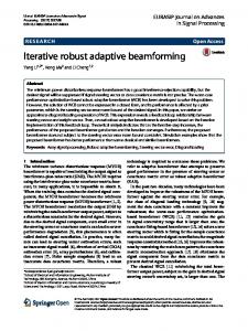
x Fig. 1.
A ULA with crossed-dipoles.
A general structure for a uniform linear array (ULA) with M crossed-dipole pairs is shown in Fig. 1, where these pairs are located along the y-axis with an adjacent distance d, and at each location the two crossed components are parallel to the x-axis and y-axis, respectively. For a far-field incident signal 1 Here
H (Hamilton) denotes the quaternion domain and R the real domain.
2
with a direction of arrival (DOA) defined by the angles θ and ϕ, its spatial steering vector is given by Sc (θ, ϕ) =
[1, e
−j2πd sin θ sin ϕ/λ
d [ n]
−
x1 [ n]
w1 [ n]
xM [ n]
wM [ n]
,
−j2π(M −1)d sin θ sin ϕ/λ T
··· ,e
]
where γ is the auxiliary polarization angle with γ ∈ [0, π/2], and η ∈ [−π, π] is the polarization phase difference. The array structure can be divided into two sub-arrays: one parallel to the x-axis and one to the y-axis. The complexvalued steering vector of the x-axis sub-array is given by { − cos γSc (θ, ϕ) for ϕ = π2 Sx (θ, ϕ, γ, η) = (3) cos γSc (θ, ϕ) for ϕ = −π 2 and for the y-axis it is expressed as { cos θ sin γejη Sc (θ, ϕ) Sy (θ, ϕ, γ, η) = − cos θ sin γejη Sc (θ, ϕ)
ϕ= ϕ=
π 2 −π 2
(4)
(5)
where q1 , q2 , q3 , and q4 are real-valued [24], [25]. In this paper, we consider the conjugate operator of q as q ∗ = q1 − q2 i − q3 j − q4 k. The three imaginary units i, j, and k satisfy ij = k, jk = i, ki = j, ijk = i2 = j 2 = k 2 = −1;
(6)
where the exchange of any two elements in their order gives a different result. For example, we have ji = −ij rather than ji = ij. For a general quaternion-valued function f (q), the df (q) derivative with respect to q can be expressed as [19], dq [21], [26] 1 ∂f (q) ∂f (q) ∂f (q) ∂f (q) df (q) = ( − i− j− k) , (7) dq 4 ∂q1 ∂q2 ∂q3 ∂q4 while the derivative of f (q) with respect to q ∗ is given by df (q) 1 ∂f (q) ∂f (q) ∂f (q) ∂f (q) = ( + i+ j+ k) . (8) dq ∗ 4 ∂q1 ∂q2 ∂q3 ∂q4 Combining the two complex-valued subarray steering vectors together, an overall quaternion-valued steering vector with one real part and three imaginary parts can be constructed as Sq (θ, ϕ, γ, η) = ℜ{Sx (θ, ϕ, γ, η)} + iℜ{Sy (θ, ϕ, γ, η)} + jℑ{Sx (θ, ϕ, γ, η)} + kℑ{Sy (θ, ϕ, γ, η)}, (9) where ℜ{·} and ℑ{·} are the real and imaginary parts of a complex number/vector, respectively. Given a set of coefficients, the response of the array is given by r(θ, ϕ, γ, η) = wH Sq (θ, ϕ, γ, η) where w is the quaternion-valued weight vector.
Fig. 2.
(10)
e[ n]
y [ n]
. . .
Reference signal based adaptive beamforming.
B. Reference Signal Based Adaptive Beamforming The aim of beamforming is to receive the desired signal while suppressing interferences at the beamformer output. When a reference signal d[n] is available, adaptive beamforming can be implemented by the standard adaptive filtering structure, as shown in Fig. 2, where xm [n], m = 1, · · · , M are the received quaternion-valued input signals through the M pairs of crossed-dipoles, and wm [n] = am +bm i+cm j +dm k, m = 1, · · · , M are the corresponding quaternion-valued weight coefficients with a, b, c and d being real-valued. y[n] is the beamformer output and e[n] is the error signal y[n] = wT [n]x[n],
Before we present the quaternion-valued steering vector model, we first very briefly review some basics about quaternion. A quaternion q can be described as q = q1 + (q2 i + q3 j + q4 k),
. . .
(1)
where λ is the wavelength of the incident signal and {·}T denotes the transpose operation. For a crossed dipole the spatial-polarization coherent vector is given by [22], [23] { [− cos γ, cos θ sin γejη ] for ϕ = π2 (2) Sp (θ, ϕ, γ, η) = [cos γ, − cos θ sin γejη ] for ϕ = −π 2
+
e[n] = d[n] − wT [n]x[n] ,
(11)
where T
w[n]
=
[w1 [n], w2 [n], · · · , wM [n]]
x[n]
=
[x1 [n], x2 [n], · · · , xM [n]] .
T
(12)
The conjugate form of the error signal is e∗ [n], given by e∗ [n] = d∗ [n] − xH [n]w∗ [n],
(13)
where {·}H is the combination of both {·}T and {·}∗ operations for a quaternion. Then w can be updated by minimizing the instantaneous square error J0 [n] = e[n]e∗ [n]. For a general quaternion-valued function f (w), the differentiation with respect to the vector w and w∗ is ∂f ∂f ∂f ∂f − i− j− k ∂a1 ∂b1 ∂c1 ∂d1 ∂f 1 . . = (14) . ∂w 4 ∂f ∂f ∂f ∂f − i− j− k ∂aM ∂bM ∂cM ∂dM ∂f ∂f ∂f ∂f + i+ j+ k ∂a1 ∂b1 ∂c1 ∂d1 1 ∂f . . = . ∂w∗ 4 ∂f ∂f ∂f ∂f + i+ j+ k ∂aM ∂bM ∂cM ∂dM
(15)
As discussed in [19], [27], the gradient of J0 [n] with respect to w∗ would give the steepest direction for the optimization surface. It can be obtained as follows 1 (16) ∇w∗ J0 [n] = − e[n]x∗ [n] , 2 and the update equation for the weight vector with step size µ is given by w[n + 1] = w[n] − µ∇w∗ J0 [n],
(17)
3
TABLE I C OMPARISON OF COMPUTATIONAL COMPLEXITY.
leading to the following QLMS algorithm [16], [17], [26] 1 w[n + 1] = w[n] + µ(e[n]x∗ [n]). 2
(18) Real-valued addition Real-valued multiplication (Including square root operation)
III. T HE RZA-QLMS A LGORITHM Using the QLMS algorithm, we can find the optimal coefficient vector in terms of minimum mean square error (MSE) and obtain a satisfactory beamforming result. However, to reduce the complexity and also power consumption of the system, in particular for a large array, we can reduce the number of sensors involved, at the cost of the final beamforming performance. To achieve this, we here derive a novel quaternion-valued adaptive algorithm by introducing an RZA term to the original cost function of the QLMS algorithm. In this way, we can simultaneously minimise the number of sensors involved while suppressing the interferences during the beamforming process. First, to minimise the number of sensors, we could add the l0 norm of the weight vector w to the cost function J0 [n] to form a new cost function Jˆ0 [n] = (1 − δ1 )e[n]e∗ [n] + δ1 ∥ w[n] ∥0 ,
(19)
where δ1 is a weighting term between the original cost function and the newly introduced term. In this way, the number of nonzero valued coefficients in w will be minimised too, where the similar idea has been applied in [28]. In practice, we could replace the l0 norm by the l1 norm. However, l1 norm would uniformly penalise all non-zero valued coefficients, while l0 norm penalises smaller nonzero values more heavily. To have a closer approximation to l0 norm, we can introduce a larger weighting term to those coefficients with smaller values and a smaller weighting term to those with larger values. This weighting term will change according to the resultant coefficients at each update of the algorithm. This general idea has been implemented as a reweighted l1 minimization [29], [30] and employed in the sparse array design problem [31], [32], [33]. The modified cost function for the proposed RZA-QLMS algorithm with the reweighting term is given by ∗
J1 [n] = (1 − δ1 )e[n]e [n] + δ1
M ∑
(εm |wm [n]|),
(20)
m=1
where εm is the reweighting term for wm . Then using the chain rule in [19], we can obtain the gradient of J1 [n] with respect to w∗ [n]. In particular, the differentiation of the second ∗ part of J1 [n] with regards to wm [n] is given by ∂(εm |wm [n]|) ∗ ∂wm ∂(|wm [n]|) ∂(|wm [n]|) 1 εm ( + i = 4 ∂am ∂bm ∂(|wm [n]|) ∂(|wm [n]|) + j+ k) ∂cm ∂dm 1 am bm cm dm = εm ( + i+ j+ k) 4 |wm [n]| |wm [n]| |wm [n]| |wm [n]| 1 wm [n] 1 = εm = εm (sign(wm [n])) , (21) 4 |wm [n]| 4
QLMS 28M+4 32M+4 (0)
ZA-QLMS 35M+4 44M+4 (M)
RZA-QLMS 38M+4 52M+4 (2M)
where sign(·) is a component-wise sign function { wm [n]/|wm [n]| wm [n] ̸= 0 sign(wm [n]) = 0 wm [n] = 0 The overall gradient result is given by 1 1 ∗ ∗ J1 [n] = − (1 − δ1 )e[n]x ∇wm m [n] + δ1 εm (sign(wm [n])). 2 4 (22) We choose the reweighting term εm as εm = 1/(σ + |wm [n]|),
(23)
with σ being roughly the threshold value below which the corresponding sensor will not be included in the update. Then, with the step size µ1 , we finally obtain the following update equation for the RZA-QLMS algorithm in vector form 1 w[n + 1] = w[n] + (µ1 − 4ρ1 )(e[n]x∗ [n]) 2 −ρ1 (sign(w[n]))./(σ + |w[n]|) , (24) where ρ1 = 14 µ1 δ1 , |w[n]| is a vector formed by taking the absolute value of the coefficients in w[n], ‘./’ is a componentwise division between two vectors, and sign(w[n]) is defined as { w[n]./|w[n]| w[n] ̸= 0 sign(w[n]) = 0 w[n] = 0 When σ + |w[n]| is removed from the above equation, it will be reduced to the ZA-QLMS algorithm in [21], with its cost function given by J2 [n] = (1 − δ2 )e[n]e∗ [n] + δ2 ∥w[n]∥1 ,
(25)
where δ2 is a trade-off factor. The update equation for the ZA-QLMS algorithm is 1 w[n + 1] = w[n] + (µ2 − 4ρ2 )(e[n]x∗ [n]) − ρ2 · sign(w[n]) , 2 (26) where ρ2 = 14 µ2 δ2 , and µ2 is the step size. We now discuss the computational complexity of the algorithms. The results are shown in Tab. I, where M is the number of vector sensors of the array. Obviously, the RZAQLMS algorithm has the highest complexity. However, as we will see in simulations, this additional cost is paid back by a resultant much smaller number of sensors, and especially at a later stage of the adaptation, when the number of sensors involved becomes smaller, the overall complexity of the RZAQLMS algorithm could be lower than the other two algorithms. After removing the sensors with a smaller magnitude for their coefficients compared to σ, the beam response difference ∆r between the original array and the new one is given by ∆r
= |wH Sq − (w − ∆w)H Sq | = |∆wH Sq | ≤ |∆wH | · |Sq | ≤ σ · ∆M ·
√ M (27)
4
10 QLMS ZA−QLMS RZA−QLMS
The beam pattern of array(dB)
−5
−10
−15
−20
QLMS ZA−QLMS RZA−QLMS
0
−10
−20
−30
−40
−25
−50
−30
Fig. 3.
0
1000
2000
3000
4000 Iterations
5000
6000
7000
−60
8000
Learning curves of the three algorithms.
where ∆M is the number of removed sensors, and ∆w is the change of w after some of its sensors are removed (the corresponding coefficients on the positions of removed sensors have a magnitude smaller than σ and are then set to zero). As a result, the maximum possible change in array response, due √ to removal of some sensors, is given by σ · ∆M · M . IV. S IMULATION R ESULTS Simulations are performed based on an array with 16 crossed-dipoles and half-wavelength spacing for the three algorithms: QLMS, ZA-QLMS and RZA-QLMS. The stepsizes µ, µ1 and µ2 are set to be 2 × 10⁻⁴ , 4 × 10⁻⁴ and 2 × 10⁻⁴ , respectively, which are chosen empirically to make sure these algorithms have a similar convergence speed. A desired signal with 20 dB signal to noise ratio (SNR) impinges from the broadside of the array (θ = 0◦ ) and two interfering signals with a signal to interference ratio (SIR) of -10 dB arrive from the directions (20◦ , 90◦ ), and (30◦ , −90◦ ), respectively. All the signals have the same polarisation of (γ, η) = (30◦ , 0). For the RZA-QLMS and ZA-QLMS algorithms, the coefficients of the zero attractor ρ1 and ρ2 are 7 × 10⁻⁷ and 2.8 × 10⁻⁵ , respectively and σ = 0.001. Their learning curves obtained by averaging results from 200 simulation runs are shown in Fig. 3 and the resultant beam patterns are shown in Fig. 4, where for convenience positive values of θ indicate the value range θ ∈ [0◦ , 90◦ ] for ϕ = 90◦ , while negative values of θ ∈ [−90◦ , 0◦ ] indicate an equivalent range of θ ∈ [0◦ , 90◦ ] with ϕ = −90◦ . First, the two nulls at the directions of the interfering signals can be observed in all three beam patterns, clearly indicating a satisfactory beamforming result for all algorithms. However, from Fig. 3, we see that although these three algorithms have a similar convergence speed, the original QLMS algorithm has the smallest steady state error, which is not surprising since it has the most degrees of freedom among them. On the other hand, the proposed RZA-QLMS algorithm has achieved a lower steady state error than the ZA-QLMS algorithm. In terms of output signal to interference plus noise ratio (SINR), it is 23.48 dB for the QLMS algorithm, 18.32 dB for the RZAQLMS algorithm, and 7.36 dB for the ZA-QLMS algorithm.
Fig. 4.
−80
−60
−40
−20
0 theta(degrees)
20
40
60
80
Beam patterns of the three algorithms.
0.15 QLMS ZA−QLMS RZA−QLMS Magnitude of Weight Coefficient
Ensemble Normalised Mean Square Error [dB]
0
0.1
0.05
0
Fig. 5.
2
4
6
8 10 Number of sensors
12
14
16
Amplitudes of the steady state weight coefficients.
The amplitudes of steady state weight coefficients for the three algorithms are shown in Fig. 5, where for the QLMS algorithm, the amplitudes of the coefficients are spread over the sixteen sensors with some small variations, while for the ZA-QLMS algorithm, some degree of sparsity has also been achieved with four of the coefficients are close to zero. However, with 0.001 as the threshold value, they can not be discarded. For the RZA-QLMS algorithm, the variation is significantly larger and seven of them are almost zero-valued, which means the corresponding sensors can be removed and only 9 sensors are needed to give a satisfactory beamforming result, rather than 16 sensors. Moreover, the difference response between the original array and the one with 7 sensors removed is extremely small, and no difference can really be observed by a naked eye, as shown in Fig. 6. Based on the steady-state sensor number, the computational complexity of the three algorithms is listed in Tab. II, where we can see that the RZA-QLMS algorithm has the lowest complexity. TABLE II C OMPARISON
OF COMPUTATIONAL COMPLEXITY IN SIMULATIONS
Real-valued addition Real-valued multiplication (Including square root operation)
QLMS 452 516 (0)
ZA-QLMS 564 708 (16)
RZA-QLMS 346 472 (18)
5
10 RZA−QLMS with 16 sensors RZA−QLMS with 9 sensors
The beam pattern of array(dB)
0
−10
−20
−30
−40
−50
Fig. 6.
−80
−60
−40
−20
0 theta(degrees)
20
40
60
80
Beam pattern of the two arrays.
V. C ONCLUSION An RZA-QLMS algorithm has been proposed for adaptive beamforming based on vector sensor arrays consisting of crossed dipoles. It can reduce the number of sensors involved in the beamforming process so that reduced system complexity and energy consumption can be achieved while an acceptable performance can still be maintained, which is especially useful for large array systems. Simulation results have shown that the proposed algorithm can work effectively for beamforming while enforcing a sparse solution for the weight vector where the corresponding crossed-dipole sensors with almost zerovalued coefficients can be removed from the system. R EFERENCES [1] H. L. Van Trees, Optimum Array Processing, Part IV of Detection, Estimation, and Modulation Theory. New York: Wiley, 2002. [2] W. Liu and S. Weiss, Wideband Beamforming: Concepts and Techniques. Chichester, UK: John Wiley & Sons, 2010. [3] C. G. Li, F. Sun, J. M. Cioffi, and L. X. Yang, “Energy Efficient MIMO Relay Transmissions via Joint Power Allocations ,” IEEE Transactions on Circuits & Systems II: Express Briefs, vol. 61, no. 7, pp. 531–535, July 2014. [4] X. C. Chen, W. Zhang, W. Rhee, and Z. H. Wang, “A ∆Σ TDCbased beamforming method for vital sign detection radar systems,” IEEE Transactions on Circuits & Systems II: Express Briefs, vol. 61, no. 12, pp. 932–936, December 2014. [5] R. T. Compton, “The tripole antenna: An adaptive array with full polarization flexibility,” IEEE Transactions on Antennas and Propagation, vol. 29, no. 6, pp. 944–952, November 1981. [6] A. Nehorai, K. C. Ho, and B. T. G. Tan, “Minimum-noise-variance beamformer with an electromagnetic vector sensor,” IEEE Transactions on Signal Processing, vol. 47, no. 3, pp. 601–618, March 1999. [7] M. D. Zoltowski and K. T. Wong, “ESPRIT-based 2D direction finding with a sparse uniform array of electromagnetic vector-sensors,” IEEE Transactions on Signal Processing, vol. 48, no. 8, pp. 2195–2204, August 2000. [8] X. M. Gou, Y. G. Xu, Z. W. Liu, and X. F. Gong, “Quaternion-Capon beamformer using crossed-dipole arrays,” in Proc. IEEE International Symposium on Microwave, Antenna, Propagation, and EMC Technologies for Wireless Communications (MAPE), November 2011, pp. 34–37. [9] X. R. Zhang, W. Liu, Y. G. Xu, and Z. W. Liu, “Quaternion-valued robust adaptive beamformer for electromagnetic vector-sensor arrays with worst-case constraint,” Signal Processing, vol. 104, pp. 274–283, November 2014. [10] M. B. Hawes, and W. Liu, “Design of fixed beamformers based on vector-sensor arrays,” International Journal of Antennas and Propagation, vol. 2015, 2015. [11] N. Le Bihan and J. Mars, “Singular value decomposition of quaternion matrices: a new tool for vector-sensor signal processing,” Signal Processing, vol. 84, no. 7, pp. 1177–1199, 2004.
[12] S. Miron, N. Le Bihan, and J. I. Mars, “Quaternion-MUSIC for vectorsensor array processing,” IEEE Transactions on Signal Processing, vol. 54, no. 4, pp. 1218–1229, April 2006. [13] N. Le Bihan, S. Miron, and J. I. Mars, “MUSIC algorithm for vectorsensors array using biquaternions,” IEEE Transactions on Signal Processing, vol. 55, no. 9, pp. 4523–4533, 2007. [14] J. W. Tao and W. X. Chang, “A novel combined beamformer based on hypercomplex processes,” IEEE Transactions on Aerospace and Electronic Systems, vol. 49, no. 2, pp. 1276–1289, 2013. [15] J. W. Tao, “Performance analysis for interference and noise canceller based on hypercomplex and spatio-temporal-polarisation processes,” IET Radar, Sonar Navigation, vol. 7, no. 3, pp. 277–286, 2013. [16] J. W. Tao and W. X. Chang, “Adaptive beamforming based on complex quaternion processes,” Mathematical Problems in Engineering, vol. 2014, 2014. [17] Q. Barth´elemy, A. Larue, and J. I. Mars, “About QLMS derivations,” IEEE Signal Processing Letters, vol. 21, no. 2, pp. 240–243, 2014. [18] W. Liu, “Channel equalization and beamforming for quaternion-valued wireless communication systems,” Journal of the Franklin Institute (arXiv:1506.00231 [cs.IT]), November 2015. [19] M. D. Jiang, Y. Li, and W. Liu, “Properties and applications of a restricted HR gradient operator,” arXiv:1407.5178 [math.OC], July 2014. [20] Y. Chen, Y. Gu, and A. O. Hero, “Sparse LMS for system identification,” in Proc. IEEE International Conference on Acoustics, Speech, and Signal Processing, Taipei, April 2009, pp. 3125–3128. [21] M. D. Jiang, W. Liu, and Y. Li, “A zero-attracting quaternion-valued least mean square algorithm for sparse system identification,” in Proc. of IEEE/IET International Symposium on Communication Systems, Networks and Digital Signal Processing, Manchester, UK, July 2014. [22] R. Compton, “On the performance of a polarization sensitive adaptive array,” IEEE Transactions on Antennas and Propagation, vol. 29, no. 5, pp. 718–725, 1981. [23] J. Li and R. Compton Jr, “Angle and polarization estimation using esprit with a polarization sensitive array,” IEEE Transactions on Antennas and Propagation, vol. 39, pp. 1376–1383, 1991. [24] W. R. Hamilton, Elements of quaternions. Longmans, Green, & co., 1866. [25] I. Kantor, A. Solodovnikov, and A. Shenitzer, Hypercomplex numbers: an elementary introduction to algebras. New York: Springer Verlag, 1989. [26] M. D. Jiang, W. Liu, and Y. Li, “A general quaternion-valued gradient operator and its applications to computational fluid dynamics and adaptive beamforming,” in Proc. of the International Conference on Digital Signal Processing, Hong Kong, August 2014. [27] D. H. Brandwood, “A complex gradient operator and its application in adaptive array theory,” IEE Proceedings H (Microwaves, Optics and Antennas), vol. 130, no. 1, pp. 11–16, 1983. [28] J. Yoo, J. Shin, and P. Park, “An improved NLMS algorithm in sparse systems against noisy input signals,” IEEE Transactions on Circuits & Systems II: Express Briefs, vol. 62, no. 3, pp. 271–275, March 2015. [29] E. J. Cand`es, M. B. Wakin, and S. P. Boyd, “Enhancing sparsity by reweighted l1 minimization,” Journal of Fourier Analysis and Applications, vol. 14, pp. 877–905, 2008. [30] W. Xu, J. X. Zhao, and C. Gu, “Design of linear-phase FIR multiplenotch filters via an iterative reweighted OMP scheme,” IEEE Transactions on Circuits & Systems II: Express Briefs, vol. 61, no. 10, pp. 813–817, October 2014. [31] B. Fuchs, “Synthesis of sparse arrays with focused or shaped beampattern via sequential convex optimizations,” IEEE Transactions on Antennas and Propagation, vol. 60, no. 7, pp. 3499–3503, 2012. [32] G. Prisco and M. D’Urso, “Maximally sparse arrays via sequential convex optimizations,” IEEE Antennas and Wireless Propagation Letters, vol. 11, pp. 192–195, 2012. [33] M. B. Hawes, and W. Liu, “Compressive sensing based approach to the design of linear robust sparse antenna arrays with physical size constraint”, IET Microwaves, Antennas & Propagation, vol. 8, issue 10, pp. 736–746, July 2014.