Progress In Electromagnetics Research, Vol. 125, 165–184, 2012
ON ADAPTIVE BEAMFORMING FOR COHERENT INTERFERENCE SUPPRESSION VIA VIRTUAL ANTENNA ARRAY W. Li1 , Y. Li1, * , and W. Yu2 1 College
of Information and Communication Engineering, Harbin Engineering University, Harbin 150001, China 2 Electromagnetic
Communication Lab, The Pennsylvania State University, University Park, PA 16802, USA Abstract—In this paper, we propose Modified Interpolated Spatial Smoothing (MISS) algorithm that solves the problem when the inhibition gain generated by Interpolated Spatial Smoothing (ISS) algorithm is not sufficiently high in virtual antenna adaptive beam forming to suppress coherent interference. Using the subspace projection concept, this paper establishes an interference subspace spanned by the interference steering vectors of the virtual antenna array, and then the interference direction information can be imported into the transformation matrix by projecting the transformation matrix into the subspace, which will make the interference components in virtual smoothing covariance matrix enhanced as it is demonstrated by theoretical analysis. Employing the Minimum Variance Distortionless Response (MVDR) beam forming method, the interference inhibition gain and Signal to Interference and Noise Ratio (SINR) performance can be significantly improved. 1. INTRODUCTION With the development and wide application of electromagnetic communication, the analyses of electromagnetic phenomena in the complex environment have become an important topic today [1]. The multi-path interference of incident signal in the practical applications is inevitable and together with intelligent interference is so-called coherent interference. The coherence between signal and interference will severely influence the performance of antenna array to receive Received 8 January 2012, Accepted 7 February 2012, Scheduled 26 February 2012 * Corresponding author: Yipeng Li (
[email protected]).
166
Li, Li, and Yu
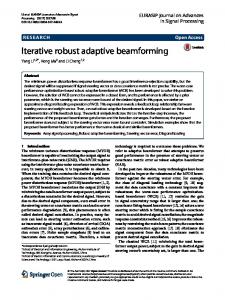
expected signals [2, 3]. In turn, this can result in signal covariance rank’s reduction and decrease the dimension of signal subspace less than the number of real signals. Furthermore, the steering vector of coherent source and noise subspace are not orthogonal anymore and the subspace approaches such as MUSIC do not work well. Spatial smoothing technique [4–6] as a common decorrelation algorithm recovers the rank of signal covariance and forces signal subspace and noise subspace orthogonal, so that the subspace approaches [7, 8] can be used effectively. It is a well-known fact that the spatial smoothing algorithm can only be applied to the antenna array with Vandermonde manifold. In Friedlander’s Virtual Array Transformation (VAT) method [9], the arbitrary shaped real antenna array can be transformed into virtual antenna array with the Vandermonde manifold by interpolating in the interested array scanning sector. The decorrlation problem in an arbitrary shaped array can be solved by applying the spatial smoothing technique through the virtual array [10–12]. Virtual array transformation can increase the degrees of freedom of an antenna array and realize the transformation between different array geometry. Therefore, VAT technique is supposed to have a broad applications in the complex environment to reduce electromagnetic interference (EMI) [13], to improve the performance of antenna array in the handhold devices [14], to adopt information from the nearby environment in the body network communication [15], to improve the imaging quality of tomography SAR [16]. In recent years, the combination of virtual antenna and array signal processing theory has drawn great attention, and most researches focus on the Direction-of-Arrival (DOA) estimation aspect [17, 18], and comparatively less in beam forming field [19]. When the Interpolated Spatial Smoothing (ISS) algorithm in [20, 21] is applied in virtual antenna adaptive beam forming, the inhibition gain cannot meet the practical requirements, and hence, the same issue happens to the output SINR of antenna array [22]. An optimum virtual array beamformer [23] employs the multiple virtual subarrays to conduct dimension recovery. In order to enhance the beam forming null and improve the anti-interference performance, we propose a Modified Interpolated Spatial Smoothing (MISS) algorithm through the modification on ISS algorithm by importing the interference direction constraint information into the transformation matrix, and adjusting a series of the consequent procedures. The interference eigenvalues obtained by the MISS algorithm become larger, and higher inhibition gain on interferers can be achieved by using MVDR beam forming method. The numerical
Progress In Electromagnetics Research, Vol. 125, 2012
167
k
(θ
)
s k (t)
ds
in
wavefront θk θk
1
d
2
...
d
N
Virtual Array Transformation 1
W1
d
2
N
WN
W2
Wopt
Figure 1. Real and virtual antenna array signal model. experiments demonstrate that the robustness of beam forming can be reinforced using the MISS algorithm and a fairly good beam preserving and null forming performance can be obtained even in the situation of small snapshots number. 2. VIRTUAL ARRAY TRANSFORMATION TECHNIQUES 2.1. Antenna Array Signal Model In this part, we introduce the real and virtual antenna array signal model as showed in Fig. 1. The real antenna array includes N elements and the distance of the array elements is d. The number of the virtual ¯ that is larger than N , and the distance of antenna array elements is N ¯ The signal sk (t) is incident from virtual antenna array elements is d. the angle θk . The weighted factors W1 , W2 , . . . , WN¯ are used to adjust the output amplitude and phase of the virtual antenna array. Considering the above array signal model, when M far field narrow band signals are incident on an antenna array, the received data X can be expressed as follows: X(t) = A(θ)S(t) + N(t)
(1)
where X(t) is N × 1 snap data vector. S(t) = [s1 (t), s2 (t), . . . , sM (t)]T
168
Li, Li, and Yu
is a vector containing the complex signal envelops of M narrowband signal sources. N(t) = [n1 (t), n2 (t), . . . , nN (t)]T is a vector of zero-mean spatially white sensor noise of variance σn2 ; A(θ) is an array manifold matrix, namely, A(θ) = [a(θ1 ), a(θ2 ), . . . , a(θM )], £ ¤T where a(θk ) = 1, ejβk , . . . , ej(N −1)βk , k = 1, 2, . . . , M represents a steering vector in the θk direction, and βk is wave number that can be represented as: 2π βk = d sin(θk ) (2) λ Assume that the signal and noise are linearly independent, then the data covariance is represented as: © ª R = E X(t)XH (t) = ARs AH + σn2 I (3) where E {·} ª denotes the mathematical expectation; Rs = © E S(t)SH (t) represents the autocorrelation matrix of signal complex envelops; σn2 is the noise power; I is the unit matrix; (·)H denotes the matrix conjugate transposition. For the coherent signal source, the rank of singular signal covariance matrix Rs will decrease to be 1. After conducting eigendecomposition on R, the dimension of signal subspace will be smaller than the rank of array manifold matrix A(θ), which will lead to the steering vector a(θk ) corresponding to the coherent signal source not orthogonal to noise subspace and the approaches based on the subspace theory getting ineffective completely. 2.2. Virtual Array Transformation Theory Virtual array transformation is based on interpolation technique [9] in which the entire antenna array scanning vector is divided into several sub-regions, and the sub-region of interest will be segmented through a certain transformation to realize the mapping from the original to virtual array. Assuming that a signal is in the region Θ, we divide Θ equally as: Θ = [θl , θl + ∆θ, θl + 2∆θ, . . . , θr − ∆θ, θr ] (4) where θl and θr are left and right boundaries of region Θ, respectively. ∆θ is step length. The real array manifold matrix in the chosen area is: A = [a(θl ), a(θl + ∆θ), a(θl + 2∆θ), . . . , a(θr − ∆θ), a(θr )] (5) where a(θi ) represents the steering vector in the θi direction of a real array, and the array manifold matrix of virtual array in the same area Θ is: ¯ = [¯ A a(θl ), ¯ a(θl + ∆θ), ¯ a(θl + 2∆θ), . . . , ¯ a(θr − ∆θ), ¯ a(θr )] (6)
Progress In Electromagnetics Research, Vol. 125, 2012
169
where ¯ a(θi ) represents the steering vector in the θi direction of a virtual array, and then there exists a fixed transformation relation B between the virtual array and the real array that satisfies: ° ° min °BA − A ¯° (7) B
F
where k·kF is Frobenius mold. When the number of interpolation ¯ is fullpoints is larger than the number of elements in real array and A rank, the transformation matrix B obtained from (7) can be expressed as: ¯ H (AAH )−1 B = AA (8) Define the transformation error is: ° ° min °BA − A ¯° B F ° ° E(B) = °A ¯°
(9)
F
Ideally, when E(B) = 0, there is no approximation in the virtual transformation process. Actually the points selected in the transformation area are finite, and there exists an approximation. If the approximation is unacceptable, we need to divide the area further and calculate the transformation matrix again. In practice, as long as the approximation is smaller than the level 10−3 , the accuracy can be ensured. The covariance matrix of virtual array can be expressed as: ¯ = BRBH = B(ARs AH + σn2 I)BH = AR ¯ sA ¯ H + σn2 BBH (10) R Through the virtual transformation, white noise received by a real array has already turned into colored noise, in order to apply numerous algorithms, we must whiten the colored noise first and get the virtual ˜ ¯ in the white noise background. Then we array covariance matrix R can apply Minimum Variance Distortionless Response (MVDR) beam forming method. The optimal MVDR weight can be obtained as follows: −1 ˜ ¯ ¯ a(θ0 ) (11) Wopt = αR where ¯ a(θ0 ) represents a virtual array steering vector in the desired ¸−1 · −1 ˜ H ¯ a(θ0 ) signal direction and the coefficient α = ¯ a (θ0 )R ¯ . 3. MODIFIED INTERPOLATED SPATIAL SMOOTHING ALGORITHM The basic concept of MISS algorithm is described as follows: Step 1 : transform a real antenna array into a virtual uniform linear antenna array;
170
Li, Li, and Yu
Step 2 : conduct forward-backward spatial smoothing technique on this virtual antenna array; Step 3: use the smoothed virtual covariance data to carry out the subsequent correlative processing. It is worthwhile to note that the virtual array transformation technique in the Step 1 has integrated the interference subspace projection process that is an obvious modification on the ISS algorithm in two steps: (i) collect the interference DOAs and establish an interference subspace according to the steering vectors of these interference DOAs; (ii) introduce the interference direction information into transformation matrix by projecting the transformation matrix to this interference subspace, which can reinforce the beam preserving and null forming performance. The smoothed virtual covariance matrix, pre-whitening colored noise process and signal steering vectors of virtual array all need to be adjusted accordingly [24]. Now, we elaborate the MISS procedure in details as follows: 1) Construct the real array signal model, calculate the covariance matrix data R and signal autocorrelation matrix RS ; 2) Do the interpolation operation in the interested array scanning ¯ area, obtain the real array manifold A and virtual array manifold A, and then calculate transformation matrix B using (8); 3) Interference subspace projection process, described as follows: Collect the interference direction information θ1 , θ2 , . . . , θM 0 by 0 the DOA estimation method [25], where M is the number of all the interferers. Then the virtual antenna array steering vector in the interferer directions ¯ a(θ1 ), ¯ a(θ2 ), . . . , ¯ a(θM 0 ) can be calculated. Establish an interference subspace spanned by these interferer steering vectors: © ª P= ¯ a(θ1 ), ¯ a(θ2 ), . . . , ¯ a(θM 0 ) (12) Define the projection matrix C as: 0 H M X (13) C= ¯ a(θi )¯ aH (θi ) i=1
Projecting the transformation matrix to the interference space, we define the new transformation matrix: ¯ = CB B (14) 4) Calculate the virtual antenna array covariance matrix according to (10), and the temporary transformation matrix has already been modified. H 2 ¯H H H H 2 H H ˜ ¯ BR ¯ B ¯ H =B(AR ¯ R= s A +σn I)B =CBARs A B C +σn CBB C ¯ sA ¯ H CH + σn2 CBBH CH =CAR (15)
Progress In Electromagnetics Research, Vol. 125, 2012
171
5) Employ the spatial smoothing technique [26] to process the virtual antenna array covariance matrix data showed in (15). At first, we need to give an introduction to the spatial smoothing algorithm. Assume that the number of signals arriving at antenna array is M , the number ¯ , the number of sub-array elements of virtual antenna array elements N m, the number of divided sub-arrays (i.e., smoothing times) p. Fig. 2 shows forward spatial smoothing algorithm. Fig. 3 shows backward spatial smoothing algorithm. ¯ = p + m − 1. Assume: From Fig. 2, we can know that N £ ¤ Fk = 0m×(k−1) |Im×m | 0m×(p−k) £ ¤ Gk = 0m×(k−1) |Jm×m | 0m×(p−k)
(16a) (16b)
where k represents the kth smoothing sub-array, Im×m a unit matrix, and Jm×m a permutation matrix whose back-diagonal elements are 1. The forward and backward spatial smoothing data covariance matrices
1
2
...
m m+1
...
N-1
N
x1(t) x2(t) x p-1 (t) x p (t)
Figure 2. Forward spatial smoothing algorithm.
1
2
...
m m+1
...
N-1 xb1(t)
b x p-1 (t)
...
x2b(t)
x pb (t)
Figure 3. Backward spatial smoothing algorithm
N
172
Li, Li, and Yu
~ R 11
~ R p1 ~ R 22
~ R
= ~ R pp
~ R 1p
N× N Figure 4. Forward-backward spatial smoothing covariance data block form. can be expressed as (17a) and (17b), respectively: p
p
X f X H ˜ ˜¯ f = 1 ˜¯ = 1 ¯ k R R Fk RF k p p k=1
b ˜ ¯ = 1 R p
p X k=1
(17a)
k=1 p
X ∗ b ˜ ˜ ¯ GH ¯k = 1 R Gk R k p
(17b)
k=1
It has already been proved that when m ≥ M and p ≥ M , the f b ˜ ˜ ¯ and R ¯ are forward and backward smoothing data covariances R both full-rank [26]. In order to reduce antenna array aperture loss and to resolve more coherent sources, in this paper we adopt forwardbackward spatial smoothing technique, and its covariance data block is shown in Fig. 4. ˜ ¯ into p × p Divide the whole virtual antenna data covariance R mutually overlapped sub-arrays. The dimension of each sub-array is m × m, then the forward smoothing covariance of the kth sub-array f ˜ ˜ ¯ k is equivalent to the kth row and the kth column block matrix R ¯ kk , R f ˜ , while the backward smoothing covariance of the ˜ =R ¯ ¯ namely, R kk
k
b ˜ ˜ ¯ k is just a processing over the block matrix R ¯ kk , i.e., kth sub-array R the forward and backward spatial smoothing deformation matrices can
Progress In Electromagnetics Research, Vol. 125, 2012
173
be rewritten as (18a) and (18b): p
X f ˜ ˜ ¯ = 1 ¯ kk R R p
(18a)
k=1
b
˜ ¯ = R
p 1X
p
³ ´∗ ˜ ¯ kk Jm Jm R
(18b)
k=1
Forward-backward spatial smoothing virtual data covariance (bf ) ˜ ¯ is the average of the forward smoothing and backward matrix R smoothing virtual covariance, as showed in (19): Ã p ! µ ¶ p ³ ´∗ X X f b 1 1 1 1 (bf ) ˜ ˜ ˜ ˜ ˜ ¯ ¯ kk + ¯ kk Jm ¯ +R ¯ = R = R R Jm R 2 2 p p k=1 k=1 µ ¶∗ p p X X f f 1 ˜ ˜ ¯k + 1 ¯ k Jm = R Jm R 2p 2p k=1 k=1 µ ¶ p p X H ∗ H 1 1 X ˜ ˜ ¯ ¯ = Fk RFk + Jm Fk RFk Jm 2p 2p =
1 2p
k=1 p X
H
˜ ¯ k + Fk RF
k=1
k=1 p X
1 2p
˜ ¯ ∗ GH Gk R k
(19)
k=1
This dovetails with the results by directly substituting the f b ˜ ˜ ¯ and R ¯ . Accordingly, the modified noise covariance expression of R matrix is: p p X X 2 H H H 1 ˜¯ (bf )= 1 F (σ CBB C )F + Gk (σn2 CBBHCH)∗ GH R k n n k k (20) 2p 2p k=1
k=1
6) Pre-whitening the colored noise: the white noise has been polluted to be colored in the transformation, and we need to carry (bf ) ˜ ¯ out pre-whitening procedure on R , obtain the virtual smoothed (bf ) ˜ ¯ covariance matrix R under the white noise background: w
(bf ) ˜ ¯w = R
µ ¶ µ ¶ (bf ) −1/2 (bf ) (bf ) −1/2 ˜ ˜ ˜ ¯ ¯ ¯ Rn R Rn
(21)
7) MVDR beam forming: according to (11), calculate the optimal (bf ) ˜ ¯ w obtained from (21). The beam forming weight Wopt using R
174
Li, Li, and Yu
temporary signal steering vector of virtual array has already become (bf ) ˜ ¯ n )−1/2 ¯ (R a(θ0 ), and the optimal weight factor is: # ¶ ¸ "µ · (bf ) −1 (bf ) −1/2 ˜ ˜ ¯n ¯w R ¯ a(θ0 ) R Wopt = "µ
(bf ) ˜ ¯n R
#H ·
¶−1/2
¯ a(θ0 )
¸ (bf ) −1 ˜ ¯w R
"µ # (22) ¶ (bf ) −1/2 ˜ ¯n R ¯ a(θ0 )
Now the optimal virtual antenna array beam forming weight of MISS algorithm is obtained. We take a comparison with the method in literature [23]. The procedure of the optimum virtual array beamformer was proposed in [23], whose construction is shown in Fig. 5. The procedure can mainly be divided into two steps: a) transform the real array into multiple virtual subarrays, carry out the spatial smoothing on Array Data X Array Data X
Virtual Subarray Interpolator
~T
1st Stage
Virtual Subarray Interpolator
i = 1,2, ... , L
i
~x ~ 1 x2
B
. . . ~ xL
Projection Matrix C
Spatial Smoothing &
Projection Process
Weight Computation
B = CB ~
x
ws
Forward/Backward Back Transformation
~T 2nd Stage
w1 w2
i
Spatial Smoothing & Prewhiten Noise
i = 1,2, ... , L
. . . wL
~
x1
~
x2
~
x3
. . .
~
xp
Combiner
g
Weight Computation
w X H
y=wx
Figure 5. Construction of optimum beamformer.
Wopt
x H y = wopt x
Figure 6. Construction of modified interpolated spatial smoothing beamformer.
Progress In Electromagnetics Research, Vol. 125, 2012
175
each virtual subarray, and then calculate the optimum weight of every subarray using each corresponding smoothed covariance matrix; b) combine each subarray weight through a certain principle, obtain the final virtual array optimum weight. Unlike the procedure described above, we apply a different virtual array configuration in the newly presented algorithm, as showed in Fig. 6, transform real array into a single virtual uniform linear array, conduct the forward-backward spatial smoothing on this virtual array directly, use the smoothed virtual covariance matrix data to calculate the optimal beam forming weight. Because we have enhanced the interference components in the virtual covariance matrix, the MISS beamformer has a higher coherent interference inhibition gain for the same input SNR, and the antiinterference performance also becomes better. 4. THEORETICAL ANALYSIS In this section, we use mathematical theory to explain the reason that MISS algorithm has a higher interference inhibition gain than that of ISS algorithm. Firstly, from (10) and (14) we know that the virtual covariance matrix after interference subspace projection can be expressed as follows: ˜ ¯ = BR ¯ B ¯ H = CBRBH CH = CRC ¯ H R (23) Substituting (23) into (19), we obtain the projected virtual covariance matrix: ¶ µ p p b f H ∗ (bf ) 1 X 1 X 1 ˜ ˜ ˜ ˜ ˜ ¯ ¯ ¯ ¯ GH ¯ R +R = Fk RFk + Gk R R = k 2 2p 2p k=1
k=1
p p ³ ´ ³ ´∗ 1 X 1 X H H ¯ ¯ H GH = Fk CRC Fk + Gk CRC k (24) 2p 2p k=1
k=1
We take forward smoothing for example to derive, and the derivation method of backward smoothing is similar. As shown in Fig. 2, we divide p sub-arrays whose number of elements is m, namely, carrying on p times smoothing on the subarrays. For the kth sub-array, the data covariance matrixes via the ISS and MISS algorithms are showed in (25): h i ¯ H ¯ f = Fk RF R (25a) k k m×m h ³ ´ i f H ˜ ˜ ¯ k = Fk RF ¯ k = Fk CRC ¯ H FH R (25b) k m×m
176
Li, Li, and Yu
According to R. O. Schmidt’s orthogonal subspace theory, we carry out an eigenvalue decomposition on the data covariance matrix ¯ f through the ISS algorithm, and we have: R k n£ £ ¤ ¤ ¯ f = Fk RF ¯ H R = 0m×(k−1) |Im×m |0m×(P −K) m×N¯ k m×m k o ¯Σ ¯U ¯ H ] ¯ ¯ · [0m×(k−1) |Im×m |0m×(p−k) ]H¯ (26) ·[U N ×N N ×m m×m
¯ is an eigenvector matrix of covariance matrix R, ¯ and the where U ¯ diagonal matrix Σ constituted by the corresponding eigenvalues is: ¯ λ1 ¯2 λ ¯ = (27) Σ .. . ¯¯ λ N
We substitute the projection matrix expression (13) into (25b) and ˜ ¯ f got also conduct an eigenvalue decomposition on covariance matrix R k via MISS algorithm, refer to Literature [27], we can get: ¢ ¤ ˜ H = £F ¡CRC ˜ f =F RF ¯ H FH ¯ ¯ R k k k k k m×m n h i o ¯Σ ¯U ¯ H ) · CH · FH = Fk · C · (U k m×m 02 ¯ M · λ1 ³ 2π d¯ 1 + e−j·2· λ sin θ1 +. . . ˜ ´2 ¯ = Fk ·U· d¯ sin θ 0 −j·2· 2π ¯2 λ M ·λ +e .. . .. . ³ ¯ H 2π d ¯ −j·2·(N−1)· λ sinθ1 H ˜ ¯ 1+e + . . . · U ·Fk ´ 2π d¯ ¯ ¯¯ +e−j·2·(N −1)· λ sin θM 0 2 · λ N m×m ˜¯ λ 1 ˜ ¯2 ˜ ˜ H H λ · U ¯ ¯ · Fk = Fk · .. U· . ˜ ¯ λN¯ m×m
Progress In Electromagnetics Research, Vol. 125, 2012
¸ ½ · £ ¤ H ˜ ˜ ˜ ¯ ¯ ¯ = 0m×(k−1) |Im×m | 0m×(p−k) m×N¯ · UΣU ¯ ×N ¯ N £ ¤H o · 0m×(k−1) |Im×m | 0m×(p−k) N¯ ×m m×m
177
(28)
˜ ˜ ˜ ¯ is the eigenvector matrix corresponding to R, ¯ Σ ¯ = where, U ˜¯ λ 1 ˜¯ λ 2 is the diagonal matrix that includes the the .. . ˜ ¯ λN¯ ˜ ¯ From (28), we can observe: eigenvalues of R. ˜¯ > λ ¯ i , i = 1, 2, . . . , N ¯ λ i
(29)
Formula (29) indicates that for the arbitrary kth smoothing subarray, the covariance matrix eigenvalues obtained from the MISS algorithm are bigger than that from the ISS algorithm. After the sum-average calculation, the eigenvalues generated from the MISS are still bigger. Similarly, we can draw the same conclusion using backward spatial smoothing method. Therefore, we can conclude that after integrating interference subspace projection operation, the virtual smoothing covariance matrix eigenvalues become larger. This is the reason, in mathematics aspect, that the nulls are deeper using MISS algorithm than the original ISS algorithm. Here MVDR beam forming method also needs to be introduced: Using the minimum variance distortionless response (MVDR) beam forming method [28], the gain in the direction of desired signal is constrained to be 1, and the array output power is ensured to be minimum. Namely, the interference and noise produce the minimum output power. Applied to the virtual array, the weighted vector of the MVDR beam forming is the solution of the following problem: h¯ ¯ i arg ¯ ¯2 WMVDR = WH ¯a(θ0 )=1 min E ¯WH X(k) =
arg H˜ ¯ WH ¯ a(θ0 )=1 min W RW
arg
(30)
where the WH ¯a(θ0 )=1 min [ ] represents the optimal solution with the minimum function value in [ ] and satisfies the equality WH ¯ a(θ0 ) = 1. arg represents an inverse function. It can be solved using Lagrangian multiplier method: −1
WMVDR =
˜ ¯ R
¯ a(θ0 ) ˜ −1 ¯ ¯ ¯ aH (θ0 )R a(θ0 )
178
Li, Li, and Yu
which dovetails with (11). The characteristic of MVDR method is that higher interference power in array generates stronger inhabitation in these directions. By introducing interference direction constraint information into the transformation matrix B with the MISS algorithm, the new eigenvalues of the covariance matrix become bigger than the conventional algorithm. The signal components corresponding to them are strengthened. Therefore, the inhibition gains in these directions will increase via the MVDR method, i.e., the nulls will be deeper as shown in the beam forming figure. 5. SIMULATION VERIFICATION Numerical experiment 1: Firstly we carry out a numerical experiment to investigate the performance of real and virtual antenna array when the number of signals arriving at array is more than system degrees of freedom. The real array is uniformly linear array of 4 elements. The element space is λ. The expected signal incidents from 0◦ direction, signal to noise ratio is SN R = 0 dB. Five independent interferers incident in −60◦ , −40◦ , 20◦ , 50◦ , 70◦ directions, and signal to interference ratio is SIR = −40 dB. The virtual antenna array is uniformly linear array of 8 elements. Element space is λ/2. Virtual transformation area is [−65◦ , −35◦ ] ∪ [15◦ , 25◦ ] ∪ [45◦ , 55◦ ] ∪ [65◦ , 75◦ ]. The step-size is 0.1◦ , and the number of snapshots is 200. Fig. 7 shows the beam forming curve via real antenna array and virtual antenna array method. In this experiment, the real array has 3 degrees of freedom, which can suppress 3 independent interferers at most. From Fig. 7, we can observe that when 5 interferers incident on the array, real array cannot generate nulls in the directions of interference; the main lobe migrates; the method gets invalid. While the virtual antenna array has 8 elements, it has 7 degrees of freedom and generates nulls in all the interference directions; the average interference inhibition gain is around −32 dB; the main lobe also points at the desired signal direction. What is slightly unsatisfactory is that the first side-lobe level (SLL) is relatively higher. We can control the side-lobe level by using Dolph-Chebyshev weighting method if necessary, but this will make the main lobe expansion. The result indicates that in this situation the virtual antenna array method is effective. In addition, it is worthwhile to further explain the following case. Ideally, no matter where the interferers and signal of interest are located, we always expect that the main lobe points at the signal of interest and adaptively generates nulls at the directions of unknown interferers. However, when the signals are incident from the
Progress In Electromagnetics Research, Vol. 125, 2012
179
normal direction of a uniformly linear array, the uniformly linear array performs the best. While its performance decreases at the directions closing to the endfire (approximately from 60 degrees, here assume that the normal direction is at zero degree), this may cause nulls drift or main lobe migration. This issue is caused by the fact that the signal subspace estimated by data samples degrades the estimation accuracy at the large incident directions in practical calculation [29]. The MISS algorithm integrates projection transformation process. After projection, the estimation error can be restrained to some extents, and the signal subspace can get enhanced, which will help weaken the performance degradation beyond of 60 degrees in the virtual beamforming figure. Numerical experiment 2: The real array is uniformly linear array of 4 elements, and the element space is λ. The expected signal incidents from 0◦ direction, and signal to noise ratio is SN R = 0 dB. Three coherent interferers lie in −60◦ , −40◦ and 50◦ directions, respectively. Signal to interference ratio is SIR = −40 dB. The virtual array is uniformly linear array of 10 elements. The element space is λ/2, and the forward-backward spatial smoothing parameter m = 6, p = 5. The virtual transformation area is [−65◦ , −35◦ ] ∪ [45◦ , 55◦ ]. The step-size is 0.1◦ . The number of snapshots is 200. Compared with real array method and interpolated spatial smoothing algorithm, we investigate the performance of the modified interpolated spatial smoothing algorithm. The beamforming curve, eigenvalue curve and 0 -5 -10
Gain(dB)
-15 -20 -25
Virtual antenna array Real antenna array
-30 -35 -40 -100
-80
-60
-40
-20 0 20 Azimuth Angle(degree)
40
60
80
100
Figure 7. Beam forming curve via real and virtual antenna array.
180
Li, Li, and Yu 0 -10 -20
Gain(dB)
-30 -40 ISS algorithm Real array method MISS algorithm
-50 -60 -70 -80 -100
-80
-60
-40
-20 0 20 Azimuth Angle(degree)
40
60
80
100
Figure 8. Coherent interferers beam forming curve using different methods. 50 Real array method ISS algorithm MISS algorithm
40
Eigenvalue(dB)
30
20
10
0
-10
1
2
3
4
5
6
7
8
9
10
Index
Figure 9. methods.
Coherent interferers eigenvalue curve using different
output SINR curve of the three methods are shown in Fig. 8, Fig. 9 and Fig. 10, respectively. In this situation, the coherent interferes cannot be inhibited via a real array method. However, because the number of virtual elements
Progress In Electromagnetics Research, Vol. 125, 2012
181
30 20
Output SINR(dB)
10 0 Real array method ISS algorithm MISS algorithm
-10 -20 -30 -40 -50
0
20
40
60
80
100 120 Snapshots
140
160
180
200
Figure 10. Coherent interferers output SINR curve using different methods. is increased, by using the spatial smoothing technique, the null can be generated in each coherent interferer direction, and the interference inhibition gain via the ISS algorithm is about −20 dB. The MISS algorithm generates about −70 dB inhibition gain, and the main lobe points at the desired signal direction. There is only one large eigenvalue in the real antenna array after the eigen-decomposition, because interferes and desired signals are completely correlated. In turn, the related signals cause the rank of signal covariance matrix RS to be 1 as discussed previously, i.e., the eigenvalues of signal subspace have “spread” into the noise subspace. The virtual antenna array integrates the spatial smoothing technique. Therefore, the rank of signal covariance matrix can be recovered, and the signal and noise subspace do not disturb each other. As the interference components get strengthened via the MISS algorithm, the gap between signal and noise subspace eigenvalues is more obvious, and the boundary is more clearly demarcated, which, in turn, can enhance the beam pattern preservation ability. Since the interferes cannot be inhibited using the real array method, its output SINR is below −30 dB; the output SINR using the ISS algorithm floats around 8 dB; the MISS algorithm generates the output SINR more than 20 dB, ensured by a high interference and noise inhibition gain.
182
Li, Li, and Yu
6. CONCLUSION In this paper, the MISS algorithm is presented which can be used to effectively solve the decorrelation problem on an arbitrary shaped antenna array. On the basis of the original ISS algorithm, it adds an additional interference subspace projection process, through MVDR beam forming, and better anti-interference performance can be obtained. Virtual antenna array output SINR is also improved. The feasibility and validity of MISS algorithm are verified by theoretical analysis and numerical experiments. REFERENCES 1. Tsang, L., J. A. Kong, and K.-H. Ding, Scatting of Electromagnetic Waves: Theories and Applications, Wiley Interscience, New York, 2000. 2. Umrani, A. W., Y. Guan, and F. A. Umrani, “Effect of steering error vector and angular power distributions on beamforming and transmit diversity systems in correlated fading channel,” Progress In Electromagnetics Research, Vol. 105, 383–402, 2010. 3. Sjoberg, D., “Coherent effects in single scattering and random errors in antenna technology,” Progress In Electromagnetics Research, Vol. 50, 13–39, 2005. 4. Shan, T. J. and T. Kailath, “Adaptive beamforming for coherent signals and interference,” IEEE Trans. on Acoustics, Speech, and Signal Processing, Vol. 33, No. 3, 527–536, 1985. 5. Shan, T. J., M. Wax, and T. Kailath, “On spatial smoothing for direction-of-arrival estimation of coherent signals,” IEEE Trans. on Acoustics, Speech, and Signal Processing, Vol. 33, No. 8, 806– 811, 1985. 6. Lu, M. and Z. He, “Adaptive beamforming for coherent interference suppression,” ICASSP, IEEE International Conference on Acoustics, Speech and Signal Processing Vol. 1, 301–304, Apr. 1993. 7. Li, Y. and H. Ling, “Improved current decomposition in helical antennas using the ESPRIT algorithm,” Progress In Electromagnetics Research,Vol. 106, 279–293, 2010. 8. Lee, J. H., Y. S. Jeong, S. W. Cho, W. Y. Yeo, and K. Pister, “Application of the Newton method to improve the accuracy of TOA estimation with the beamforming algorithm and the MUSIC algorithm,” Progress In Electromagnetics Research, Vol. 116, 475– 515, 2011.
Progress In Electromagnetics Research, Vol. 125, 2012
183
9. Friedlander, B., “The root-music algorithm for direction finding with interpolated arrays,” Signal Processing, Vol. 30, No. 1, 15– 29,1993. 10. Friedlander, B. and A. J. Weiss, “Direction finding using spatial smoothing with interpolated arrays,” IEEE Transactions on Aerospace and Electronic Systems, Vol. 28, No. 2, 574–587,1992. 11. Lau, B. K., G. J. Cook, and Y. H. Leung, “An improved array interpolation approach to DOA estimation in correlated signal environments,” ICASSP, Proceedings of IEEE International Conference on Acoustics, Speech and Signal Processing, Vol. 2, 237–240, 2004, 12. Lau, B. K., M. Viberg, and Y. H. Leung, “Data-adaptive array interpolation for DOA estimation in correlated signal environments,” ICASSP, Proceedings of IEEE International Conference on Acoustics, Speech and Signal Processing, Vol. 4, 945–948, 2005. 13. Zhao, X. W., X. J. Dang, Y. Zhang, and C. H. Liang, “The multilevel fast multipole algorithm for EMC analysis of multiple antennas on electrically large platforms,” Progress In Electromagnetics Research, Vol. 69, 161–176, 2007. 14. Chiu, C. W., C. H. Chang, and Y. J. Chi, “Multiband folded loop antenna for smart phones,” Progress In Electromagnetics Research, Vol. 102, 213–226, 2010. 15. Gemio, J., J. Parron, and J. Soler, “Human body effects on implantable antennas for ism bands applications: Models comparison and propagation losses study,” Progress In Electromagnetics Research, Vol. 110, 437–452, 2010. 16. Ren, X. Z., L. H. Qiao, and Y. Qin, “A three-dimensional imaging algorithm for tomography SAR based on improved interpolated array transformation,” Progress In Electromagnetics Research, Vol. 120, 181–193, 2011. 17. Yang, P., F. Yang, and Z.-P. Nie, “DOA estimation with subarray divided technique and interpolated esprit algorithm on a cylindrical conformal array antenna,” Progress In Electromagnetics Research, Vol. 103, 201–216, 2010. 18. Park, G.-M., H.-G. Lee, and S.-Y. Hong, “DOA resolution enhancement of coherent signals via spatial averaging of virtually expanded arrays,” Journal of Electromagnetic Waves and Applications, Vol. 24, No. 1, 61–70, 2010. 19. Yang, P., F. Yang, Z.-P. Nie, B. Li, and X. Tang, “Robust adaptive beamformer using interpolation technique for conformal antenna array,” Progress In Electromagnetics Research B, Vol. 23, 215–228,
184
20. 21.
22. 23. 24.
25. 26.
27. 28. 29.
Li, Li, and Yu
2010. Weiss, A. J. and B. Friedlander, “Performance analysis of spatial smoothing with interpolated arrays,” IEEE Transactions on Signal Processing, Vol. 41, No. 5, 1881–1892, May 1993. Weiss, A. J. and B. Friedlander, “Performance analysis of spatial smoothing with interpolated arrays,” IEEE International Conference on Acoustics, Speech and Signal Processing, Vol. 2, 1377–1380, 1991. Su, B.-W., “Research on array digital beamforming technology (in Chinese),” Doctoral Dissertation, 39–55, National University of Defense and Technology, 2006. Lee, T.-S. and T.-T. Lin, “Adaptive beamforming with interpolated arrays for multiple coherent interferers,” Signal Processing, Vol. 57, No. 2, 177–194, Mar. 1997. Li, W., Y. Li, L. Guo, W. Yu, and R. Mittra, “Adaptive beamforming technique for virtual antenna using Modified Interpolated Spatial Smoothing algorithm,” PIERS Online, Vol. 7, No. 7, 617–620, 2011. Zhang, X., J. Yu, G. Feng, and D. Xu, “Blind direction of arrival estimation of coherent sources using multi-invariance property,” Progress In Electromagnetics Research, Vol. 88, 181–195, 2008. Pillai, S. U. and B. H. Kwon, “Forward/backward spatial smoothing techniques for coherent signal identification,” IEEE Transactions on Acoustics, Speech, and Signal Processing, Vol. 37, No. 1, 8–15,1989. Li, W., Y. Li, L. Guo, and W. Yu, “An effective technique for enhancing anti-interference performance of adaptive virtual antenna array,” ACES Journal, Vol. 26, No. 3, 234240, 2011. Souden, M. and J. Benesty, “A study of the LCMV and MVDR noise reduction filters,” IEEE Transactions on Signal Processing, Vol. 58, No. 3, 4925–4935, 2010 Buhren, M., M. Pesavento, and J. F. Bohme, “Virtual array design for array interpolation using differential geometry,” ICASSP’04, Vol. 2, No. 2, 229–232, 2004.