Adaptive Beamforming using the Reconfigurable - Semantic Scholar

Adaptive Beamforming using the Reconfigurable M ONTIUM TP Marcel D. van de Burgwal, Kenneth C. Rovers, Koen C.H. Blom, André B.J. Kokkeler, and Gerard J.M. Smit Faculty of Electrical Engineering, Math and Computer Science University of Twente Enschede, The Netherlands Email: {m.d.vandeburgwal, k.c.rovers, k.c.blom, a.b.j.kokkeler, g.j.m.smit}@utwente.nl

Abstract—Until a decade ago, the concept of phased array beamforming was mainly implemented with mechanical or analog solutions. Today, digital hardware has become powerful enough to perform the massive number of operations required for real-time digital beamforming. While more and more applications are using beamforming to improve the communication channel utilization both in space and frequency, many dedicated digital architectures are proposed for the processing. By using a reconfigurable architecture, the same hardware platform can be reused for different applications with different processing needs. In this paper, we present a reconfigurable Multi-processor System-onChip based solution for phased array processing that supports advanced tracking mechanisms to continuously receive signals with a mobile receiver. An adaptive beamformer for DVB-S satellite reception is presented, that uses a Constant Modulus Algorithm to track satellites. The processing of a receiver with 64 antennas and 3 beams is mapped on a reconfigurable processor named M ONTIUM TP. The total implementation of such a receiver requires about 570 clock cycles on a single M ONTIUM TP, but can also be partitioned over multiple M ONTIUM TPs to support larger phased arrays. Index Terms—Adaptive beamforming; phased array; reconfigurable processor; MPSoC

I. I NTRODUCTION Phased array beamforming techniques have been used in radar systems for many years already. The design of these systems is mainly driven by functional requirements (e.g., resolution, sensitivity, response time) where non-functional requirements (e.g., costs, power consumption) are of secondary concern [1]. For that reason, no low-cost, low-power phased array systems are available yet. However, in areas like software defined radio and for satellite receivers, phased array antennas show great promise but their large scale introduction has been obstructed by the high costs involved. Our goal is to develop a low-cost, low-power phased array receiver platform. This can be realized by using a scalable architecture that is flexible enough to support multiple applications, such that the same architecture can be reused for more applications. Reconfigurable Multiprocessor System-on-Chip (MPSoC) based architectures seem to be promising, as they offer high performance (by enabling parallel processing through multiple processors) and are flexible within a certain application domain (reconfiguration enables efficient reuse of hardware by reconfiguring parts of an application). Conventional phased array receivers typically use a large amount of dedicated central processing hardware, making

Beamformer RF

wa v

ef

AP

ψc

+

ron t RF

AP

ψc

RF

AP

ψc

d ∆l

BS

DOA Beam control

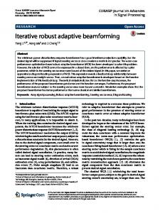
Fig. 1.

Generic phased array receiver

the system neither scalable nor power efficient [2]. After an introduction to phased array systems and their different applications in Section II, we will provide a more thorough discussion on the required processing and its complexity in Section III. The processing is mapped to a tiled architecture using reconfigurable processors (presented in Section IV). Next, we will show how the algorithm is implemented in Section V. II. P HASED ARRAY SYSTEMS AND APPLICATIONS The system blocks of a generic phased array system are shown in Fig. 1. In a phased array receiver, signals are received at multiple antennas. After the Radio Frequency (RF) front end for each antenna, Antena Processing (AP) is applied for calibration or equalization purposes (to correct for electrical or mechanical distortions of the front-end and the wireless channel). The signals are then combined by the beamforming processing (beamformer) to create a resulting signal with for example a maximum sensitivity in a direction of interest or a minimum sensitivity (a null) in the direction of an interfering signal. Beamsteering (BS) refers to changing the shape and direction of the formed beam by changing the gain and delay of the antenna signals before summation. Assume the phased array consists of antennas placed at a distance d apart, while a wavefront arrives at an angle ϑ incident

TABLE I OVERVIEW OF APPLICATIONS WHERE BEAMFORMING CAN BE BENEFICIAL

DVB-S # Antennas # Beams Frequency (GHz) Bandwidth (MHz) SNR (dB) AD bits

256 3 10–13 50 16 4

Radar 4096 20 7–13 100 100 16

Radio astronomy 8672 24 0.4–2.8 100 70 12

Wireless base stations

to the array. The wavefront travels a distance ∆l = d · sin (ϑ) further to the next antenna, which results in a time delay ∆t = ∆l c between the signals (where c is the propagation speed of radio waves). If the signal is a narrowband signal, this time delay results in a phase shift (∆ψ = ω · ∆t) giving rise to the term ‘phased array’. By correcting the delay, the direction of maximum sensitivity is steered [1].

AD AD AD conversion conversion conversion

Equalization Equalization Equalization

Beam forming Beam forming

Antenna processing

Matched filter Matched filter

QPSK demapping QPSK demapping Baseband processing

Beam steering Beam steering

64 32 2–6 10-100 30 10

Figures for radar, radio astronomy and wireless base stations are based on current requirements and extrapolated to the near future.

A. Applications

RF RF RF frontend frontend frontend

DOA estimation Beam control

Fig. 2.

Main system blocks in the phased array receiver

antenna processing. Furthermore as the received signals are very weak, low noise figures are important. 4) Wireless base stations: During the last few years, multiantenna techniques have been included in new Software Defined Radio (SDR) standards. Such Multiple Input/Multiple Output (MIMO) systems allow for higher channel utilization, as their transmission techniques are designed for both spatial and spectral optimization. Beamforming is one of the techniques that can be used to optimize the spatial use of the spectrum. Nowadays, receivers typically use 2 or 3 antenna elements at most. Adding more antenna elements implies that multiple additional front-ends are to be included, which makes a portable receiver less compact and efficient. For the base station, however, beamforming is a useful technique as the transmitted power can be spatially controlled such that the beam is focused at receivers. Additionally, the same spectrum may be reused spatially by steering a beam to each receiver.

Beamforming can be beneficial for any RF system, such as Digital Video Broadcast for Satellite (DVB-S), radar, radio astronomy and wireless communications. A cost-effective solution could be to design a single generic beamforming architecture that is flexible and modular such that each of these applications could be supported. Therefore, a comparison of the requirements of these applications is given in Table I. 1) DVB-S: The DVB-S [3] standard specifies a frequency of 10.7 to 12.75 GHz, a Signal to Noise Ratio (SNR) of 16 dB, III. P HASED ARRAY PROCESSING AND COMPLEXITY a channel bandwidth of 36 MHz (effective bandwidth used is In a dynamic environment where transmitters are continu50 MHz due to pulse shaping filter roll-off) and satellites are at ously moving with respect to the array, adaptive processing is least 5◦ apart. Conventional dish-based systems must be steered required to detect and follow transmitters. One example would mechanically.This makes the dish unsuitable for mounting on be the application of the DVB-S satellite receiver mentioned vehicles that are moving, such as cars or yachts. A phased array in section II mounted on a vehicle, for example on the roof of system can therefore be beneficial. Broadcasts from multiple a car or on the cabin of a yacht. Fig. 2 shows the phased array satellites can be received simultaneously by enabling for two or processing chain that is used for the DVB-S reception case. three independent beams. This is useful, when multiple users For each of the blocks in the chain after the AD conversion, want to receive signals from different satellites simultaneously. we will shortly describe functionality and complexity. 2) Radar: Radar is a specialized application aimed at detecting and locating reflecting objects or targets. It is for example used for scanning and tracking or guiding objects. A. Antenna processing Future phased array radar systems require a large array size For accurate beamforming, it is important that the gain and (a few thousand antennas), a high SNR (100 dB) and a delay of each antenna up to the beamforming is equal. To high sample rate (200 MHz). A suitable band for realizing realize this, antenna calibration and/or channel equalization systems with such spectral bandwidth requirements is the region has to be applied. This can be implemented by an (Feq − 1)th between 7 to 13 GHz. At each moment in time, there might order Finite Impulse Response (FIR) filter, where the minimum be multiple interesting objects in sight. Therefore, a typical order can be determined based on the required SNR and filter tracking radar should be able to track tens of objects, which roll-off. For each filter tap, one multiply-accumulate has to requires as many independent beams. be calculated. Hence, the total computational complexity of 3) Radio Astronomy: The aim of radio astronomy is to one FIR filter equals Feq multiply-accumulates. As a filter is produce images of celestial objects. As the objects of interest needed for each antenna, the amount of processing can easily are very distant, the beam width must be as narrow as possible. become as large as the beamforming itself. However, it is This requires a very large array with accurately calibrated independent of the number of beams that are formed.

u2

B. Beamforming To implement phase shifting in the digital domain, a FIR filter can be used, which consists of complex multiplications followed by addition. In the narrowband case, a single complex multiplication for each antenna can be used. The phase delay correction with a complex multiplication has the advantage that it is flexible with respect to the beam-shape and its angle. In case of multiple beams, each beam can be pointed in a different direction independently, while its shape may differ from other beams. However, the costs for this flexibility are large as processing costs are constant per beam. C. Baseband processing The modulation technique used in DVB-S for transmitting symbols is Quadrature Phase Shift Keying (QPSK) [3]. QPSK modulation maintains a constant modulus, while the information is added by appling a multiple of π2 shift in phase to the carrier frequency. When switching instantaneously between two symbols, high frequency components occur in the transmitted signal due to discontinuity in the phase. The transmitter uses a pulse shaping filter to compress the signal into a slightly wider frequency band. At the receiving side, a matched filter is then used to decompress the signal such that the modulation information is reconstructed. The matched filter can be implemented using a FIR filter consisting of Fmf taps. Since this filter is applied to the output of the beamformer, its complexity only depends on the number of beams B. D. Beam control

2 +

2

|u| y [n]

∠u

−

× ×

sin (u)

4 ×

Re Im

C

−

u1 u2

1 µ

~x [n]

Fig. 3.

~ [n] φ +

×

−

~ [n + 1] φ

Block diagram of the CMA adaptive beamsteering algorithm

avoided. Direction of Arrival is not in scope of this article and therefore, for the remainder of this article we will assume that initial locations of transmitters are known. Once the initial locations of the satellites are known, a tracking algorithm is enabled. As mentioned in the previous section, QPSK is used for transmitting DVB-S symbols. This modulation technique has well-defined structural and statistical properties. The signal is modulated in phase only, which is a strict structural property. The highest utilization of the channel can be reached when the usage of all constellation points is uniformly distributed, so transmitted symbols have a clear statistical property. Since the gain is assumed to be constant, a so-called Constant Modulus Algorithm (CMA) can be used efficiently [7]. Xu proposed an extension to CMA that allows for correction of phase deviations [8]. CMA uses both the antenna samples (~x) as well as the output of the beamformer ~ ∗ ~x) to adjust the current steering vector (φ) ~ such that (y = φ the modulus error of the beamformer output with respect to the expected modulus used by QPSK is minimized. This is done by applying an iterative gradient descent method to decrease the cost function J, which is given by Equation 1:    2
~ = E |y|2 − 1 + E sin2 (26 y) J φ (1)

The pointing direction and shape of the beam are steered by the beam control part. Since the receiver is continously moving, an adaptive beamsteering algorithm is required. There are 3 classes of adaptive beamsteering algorithms [4]. Spatial beamforming algorithms use correlation between the data streams received by individual antennas. This requires a considerable amount of processing, as the correlation may be done over long data streams and over multiple antennas. Algorithms of the temporal beamforming class rely on correlation between This can be rewritten to (2) [8]: the received data stream and a known reference stream. For ~ [n + 1] = φ ~ [n] − µ∇ ~ J example, when multi-path effects can occur, often pilot symbols φ φ   are added to synchronize with the received signal. The third 4 2 + 4 sin (46 y) 8j |y| − |y| class consists of so-called blind beamforming algorithms. These ~ [n] − µ · = φ · ~x algorithms use structural or statistical properties of the received 4j · y signal to correct the beam direction. (2) In the initial situation where the satellites have not been After optimization, we get: detected yet, a search action has to be done to find the location   4 2 of possible transmitters. This can be done with a so-called 2 |y| − |y| − j sin (46 y) ~ [n + 1] = φ ~ [n] − µ · φ · ~x (3) Direction of Arrival (DOA) estimation algorithm. Since there y is no reference signal available in the initial situation, only a spatial beamforming algorithm can be used for DOA estimation. which is also shown in Fig. 3. CMA scales linearly with the number of antennas N , Examples of suitable DOA algorithms are ESPRIT [5] and ~ are vectors of length N . The calculation because ~x and φ MUSIC [6]. The disadvantage of these algorithms is their high 4 2
2 |y| −|y| −j sin(46 y ) ( ) complexity of O N 4 (where N is the number of antennas) of µ · only consists of scalar operations y due to the correlation operations calculated for all possible and therefore requires a fixed number of operations. ~ the beam pattern tracks the antenna pairs. Therefore, a real-time implementation of such Using the steering vector φ, algorithms is very computational intensive and should be transmitter while interferers are automatically suppressed.

TABLE II C OMPLEXITY PER BASIC OPERATION

Antenna processing Beamforming Beam steering Baseband processing

Operation

Complexity

Equalization Phase shift CMA Matched filter

O (N Feq ) O (N B) O (N B) O (BFmf )

PPA M01

A

M02

B

C

ALU1 OUT2

Memory decoder

Multiple transmitters can be tracked by adding a CMA algorithm for each transmitter. As a result, the total complexity for tracking B beams with CMA equals O (N B).

D E

OUT1

M03

A W

M04

B

C

ALU2

OUT2

D E

OUT1

Interconnect decoder

M05

A W

M06

B

C

ALU3

OUT2

Register decoder

D E

OUT1

M07

A W

M08

B

C

ALU4

OUT2

D E

OUT1

M09

A W

M10

B

C

D

ALU5

OUT2

OUT1

ALU decoder

Sequencer

Network Interface

E. Algorithm complexity An overview of the complexity of the antenna processing and beamforming is given in Table II. The table shows the parameter dependencies for the figures mentioned in the previous sections.

Fig. 4.

Montium Tile Processor

1) Program control: Inside the M ONTIUM TP, shown in Fig. 4, three regions can be identified. The lower region consists Phased array processing can be characterized as a streaming of a sequencer in which the kernel is stored. It contains a application with high data rates and processing requirements, programmable Static Random Access Memory (SRAM) to but a regular processing structure. Because of costs, complexity, store the kernel instructions. A program counter is used for the dependability and scalability reasons a design with mostly program flow. It is directly connected to the SRAM to select identical components is preferred. Because a scalable and the next instruction to be executed. Hence, an instruction can regular solution is needed, a tiled reconfigurable architecture be fetched immediately as it is not affected by typical memory is proposed [9]. We aim at a processing architecture which is access delays as encountered in conventional architectures. As flexible enough to support multiple methods of beamforming there is no interaction between the data path and the instruction (based on phase shifting, time delay or Fast Fourier Transform program, the kernel execution is fully deterministic. (FFT)), as well as beamsteering and beam-control. 2) Configuration memory: The instruction selected by the A reconfigurable processing array provides flexibility and sequencer is decoded by a number of decoders. A memory has a number of advantages. For example, we can use only decoder decodes the instruction that is used to generate the part of the array or create multiple sub-arrays to save energy address patterns for the memories in the data path. The or increase the lifetime. Moreover, graceful degradation is interconnect decoder decodes the part of the instruction provided since individual tiles in a reconfigurable architecture required to control the crossbar and local buses around the might fail due to aging. Reconfigurability inherently leads to an ALUs and the memories. The selection of ALU operands in adaptable system, that can be adapted to changing environments the register file is done byu the register decoder and the ALU while maintaining the quality of service. instruction itself is decoded using the ALU decoder. 3) Processing Part Array: The decompressed instructions A. Montium Tile Processor that are generated by the decoders are sent to the upper region, The M ONTIUM TP is an example of a coarse-grained the Processing Part Array (PPA). It consists of 5 identical 1 reconfigurable processor [10] developed by Recore Systems . ALUs together with a local interconnect and a large crossbar The M ONTIUM TP targets the Digital Signal Processing (DSP) consisting of 10 global buses that provides a high bandwidth algorithm domain. Several core operations (called kernels) used to 10 memory units. Each ALU can be connected to two of the in DSP applications like baseband processing and channel memories via a local interconnect or to the 8 other memories decoding in wireless communications receivers have been via the global buses. The operands for the ALU are stored in efficiently mapped on the M ONTIUM TP architecture [11]. 4 register files which can be read simultaneously. In addition, It is typically used in multi-processor systems, for example in each ALU can receive an intermediate value from its right the Annabelle MPSoC [12]. Its template based design allows neighbor ALU via an east-west connection. Using these 5 for customization of architectural properties like data path inputs, multiple operations can be executed simultaneously and width (16-bit by default), targeted clock frequency (100 MHz from each ALU at most 3 results can be sent to the west output for 90nm technology) and processing capacity (5 parallel Arithmetic Logic Units (ALUs) for the reference design). This and both outputs connected to the interconnect respectively. reference design has a silicon area of approximately 2 mm2 Fig. 5 shows the internal structure of one ALU. The upper part, level 1, contains 4 function units, each and a power consumption of approximately 550µW/MHz. of which can execute bitwise and logic operations or simple 1 http://www.recoresystems.com arithmetic operations. Each function unit generates status flags IV. R ECONFIGURABLE TILED ARCHITECTURES

A

B

C

function unit 1

D

ALU performance is optimized. Per memory, the M ONTIUM TP contains an Address Generation Unit (AGU) that provides the hardware support for memory addressing.

function unit 2

Level 1 function unit 3 A Z1 A

B

V. I MPLEMENTATION AND R ESULTS

function unit 4

dec

SB

C Z1 B

mX

D

mY

× Level 2

Z1 A Z1 B

B

D

east SB

+ west ZA

B

D mB

+

Level 3 Z1 A

Fig. 5.

−

Z1 B

Z1 A

mO1

mO2

o1

o2

Z1 B

Structure of one M ONTIUM TP ALU

In the previous sections, we presented the algorithms that were selected for phased array processing. As can be seen in Fig. 2, the antenna processing needs to be performed for both the beamforming and beam control. By using reconfigurable hardware, the beamforming and beamsteering functionality can be replaced temporarily by DOA estimation. Here we present the implementation of beamforming and tracking, with the assumption that the initial positions of transmitters are known. As shown in [13], the update rate of the beam control algorithms can be decreased considerably before symbol errors start to occur. Therefore, for the remainder of this article we 1 assume a beam update rate of ρ = 250 = 0.004 updates per antenna sample. We mapped the digital beamsteering and beamforming to an MPSoC architecture based on the M ONTIUM TP architecture as presented in Section IV and observed the processing requirements for a DVB-S receiver using N = 64 antennas. The antenna signals are sampled by 50 MHz I/Q ADCs, such that they produce 50 Msamples/s. Antenna front-end errors are corrected by an equalization filter, which is implemented by a complex FIR filter of Feq = 5 taps.

to indicate the occurrence of overflow, a negative result or whether its result equals zero. These status flags may be used by the sequencer, for example for conditional jumps. In the A. Antenna processing and beamforming second level a Multiply Accumulate (MAC) operation can be The complex FIR filter required to implement the equalizaexecuted. Its multiplier operates on either the outputs of the tion filter can be executed on the M ONTIUM TP in 5 clock first level, named Z1 A and Z1 B, or the register files A to D. cycles per sample per antenna (i.e. one tap mapped on 4 Next, the operands for the adder can be selected from the result multipliers) [14]. So, in total for all antennas 64 ∗ 5 = 320 of the multiplication, the register files A to D, the outputs of clock cycles are required. The beamforming operation requires level 1, or the east input. In addition, depending on the value one complex multiplication and one addition per beam per of the status bit (SB), the right operand for the adder can be sample per antenna (which can be executed in 1 clock cycle dynamically selected from inputs B, D, Z1 A and Z1 B. The for the M ONTIUM TP), so 64 clock cycles per beam. Hence, output of the adder is made available to the next ALU at the left for 3 beams the antenna processing and beamforming together side through the west output and can be used in the butterfly can be executed in 320 + 3 ∗ 64 = 512 clock cycles per sample. unit located in the lower part of the ALU. Two results can be Luckily, almost all operations can be done in parallel. Therefore, returned via outputs o1 and o2 . the 512 clock cycles required to process one sample can be Since the ALU is not pipelined, the entire operation from the divided over multiple M ONTIUM TPs. Since the M ONTIUM register file inputs to the ALU outputs can be done within one TP can execute 2 instructions per sampling period, at least 256 clock cycle. Almost all arithmetic operations in the ALUs can M ONTIUM TPs are required to enable real-time processing. be executed in either integer modus (i.e., they operate on the 16 rightmost bits) or in 1.15 fixed point modus (i.e. the leftmost B. Baseband processing bit is used as sign bit whereas the other bits contain the fixed The matched filter is implemented using two Fmf = 9 point fraction). In order to avoid overflow, the intermediate taps FIR filters for the I and Q parts of the beamformer values can be saturated. Many DSP applications are based on vector or matrix output. Hence, for 3 beams this part of the baseband requires operations. Hence, the memory addressing can be done in 3 ∗ 2 ∗ 9 = 54 MAC operations per antenna sample. a regular way. Typically, these addressing patterns consist of linear addressing, stride-by-n (i.e., the address is incremented C. Beam steering by n after each read or write operation), bit reversing (an output A schematic overview of the CMA algorithm is given in reordering technique that is typically used for FFT algorithms) Fig. 3. Some arithmetic operations can be mapped on the and modulo counting (e.g. for creating circular buffers). By M ONTIUM TP ALUs directly, but three operations are required supporting these operations in hardware, the address calculation which do not directly fit. These operations are explained in the can be done separately from other ALU operations such that the following sections.

1) Transforming Cartesian coordinates to polar coordinates: The conversion from Cartesian coordinates (x, y) to polar coordinates (r, θ) and back requires some goniometric operations. These could be implemented by a large Lookup Table (LUT), at the consequence of a limited accuracy. A more efficient and accurate approach is the COordinate Rotation DIgital Computer (CORDIC) algorithm [15]. We mapped the algorithm, as described in [16], to the M ONTIUM TP. For the conversion from Cartesian to polar coordinates, the vectoring mode is used. The equations for the vectoring mode are: xi+1 = xi − yi · di · 2−i

yi+1 = yi + xi · di · 2−i

yi

i

A

B

D

A

B >>

neg

neg

1

0

C

yi

tan−1 2−i

D

A




B

yi

zi

C

D

i operation. For yi+1 and zi+1 , di is determined explicitly by the sign of yi . Both the positive and negative values are calculated for the left operand. For example, for calculating xi+1 the value of yi · 2−i and its negative value are both calculated and based on the the decision variable  di one of them is subtracted from xi . The values for tan−1 xy00 are calculated offline and stored in a read-only memory. During the calculation of the CORDIC equations, an AGU reads the memory and writes the read value to the register file for ALU 3. Hence, reading these constants does not require any additional clock cycles. Using this mapping, all three CORDIC equations can be calculated in a single clock cycle. The results of the implemented algorithm are shown in Fig. 7. As can be seen in Fig. 7, each iteration yields one additional bit of precision. Due to the bitshift operations and the limited word-width of the M ONTIUM TP, the smallest possible error is reached after 14 iterations. The CORDIC equations Equation 4 to Equation 6 are only valid for rotation angles between − π2 and π2 . For larger angles, an initial rotation over ± π2 should be applied, which can be realized with a set of equations that is slightly different from Equation 4 to Equation 6. The M ONTIUM TP implementation of the initial

yi+1

ALU 1

Fig. 6.

zi+1

ALU 2

ALU 3

Mapping of CORDIC equations on 3 M ONTIUM TP ALUs

0 Gain error Angle error

−2 −4 Accuracy (bit index)

yn = 0

xn An

i

>>

where di = +1 if yi < 0, −1 otherwise. When the number of iterations n is increased, the final values will approximate to: q (7) xn = An x20 + y02 y0 zn = z0 + tan−1 x0 Yp 1 + 2−2i An =

xi

(4)

zi+1 = zi − di · tan−1 2



C

xi

−6 −8 −10 −12 −14 −16 1

2

3

4

5

6

7

8 9 10 CORDIC iteration

11

12

13

14

15

16

Fig. 7. Error between M ONTIUM TP result and input value (in bits) after each CORDIC iteration

equations is comparable to the mapping presented for the regular CORDIC operations Equation 4 to Equation 6. Hence, the calculation of the initial equations can be done in one additional iteration. 2) Sine calculation: The sine function could be calculated very accurately using CORDIC. However, this requires an additional CORDIC operation which is expensive in terms of clock cycles. Instead, we chose to map the sine function to a LUT which is stored inside one of the memories. The upper 10 bits of the 16-bit fixed point angle are used as address for the lookup. Such a lookup only requires 2 clock cycles, which is much less compared to running a complete CORDIC operation. 3) Complex division: The complex division could be implemented by using 2 CORDIC operations, one real division and 2 multiplications [17], which is useful for implementation at multiplier-limited architectures. The M ONTIUM TP, however, contains multipliers and therefore, more efficient implementations of the complex division can be made. Assume a division between the complex numbers X = a + jb and Y = c + jd. The division can be rewritten as follows: a + jb a + jb c − jd ac + bd bc − ad = · = 2 +j 2 2 c + jd c + jd c − jd c +d c + d2

(11)

TABLE III R EQUIRED M ONTIUM TP CLOCK CYCLES PER INPUT SAMPLE USING 64 ANTENNAS AND FORMING 3 BEAMS

1.4

saturated value

1.2

Operation

µ/|y|2

1

Antenna processing Beamforming Beam steering Baseband processing

0.8

0.6

0.4

Equalization filter Phase shift CMA Matched filter Total

†

0.2

µ 0 0

0.2

µ

0.4

0.6

0.8

Clock cycles 320 196 ρ ∗ 288† 54 570 + ρ∗288

CMA implementation costs are 288 clock cycles when updated for each antenna sample. However, for a realistic update rate ρ = 0.0004, the cost per beam update is less than one clock cycle.

1

|y|2

Fig. 8.

Contents of the LUT for calculation of

Now define e =

1 c2 +d2 .

µ |y|2

After substitution in (11), we get:

a + jb = . . . = (ac + bd) · e + j (bc − ad) · e c + jd

2048 bytes, whereas the tan−1 read-only memory used for CORDIC takes 32 bytes of memory space. These tables can be loaded in 41 µs. Hence, in less than 50 µs the M ONTIUM TP is ready for execution.

(12)

which can be implemented by 6 multiplications, 2 additions and the costs for the calculation of e. 1 1 Note that e = c2 +d . For the division used in (3), 2 = |Y |2 X corresponds with the nominator and Y corresponds with the denominator which is y, so e = |y|1 2 . As can be seen

VI. R ELATED WORK

Many reconfigurable beamforming architectures are based on bit-level programmable Field Programmable Gate Arrays (FPGAs), like [18], [19], which perform very good as they can be optimized to the application. However, configuration times 2 in Fig. 3, the calculation of |y| is already done. Its inverse are long (milli-second to second scale), so no processing is can be calculated efficiently by using a LUT, similar to the possible during that period. The reconfigurable tiled architecture 2 1 sine calculation. The values of |y|2 with |y| ∈ [0, . . . , 1i are approach used in this paper can be reconfigured much faster in the range of h1, . . . , ∞i, which cannot be represented in (nano-second to micro-second scale), where it is possible to a 1.15 fixed point notation. A straight-forward LUT based reprogram individual processors instead of the entire chip. The implementation is therefore not useful. In order to solve this RaPiD reconfigurable architecture [20] has some similarities problem, the multiplication by a step factor µ (see Fig.3) is compared to the M ONTIUM TP, but it is not designed as included in the LUT. Typically, µ = 0.005 is used for the a tile processor. The reconfigurable beamformer processor best tracking results. So, instead of using a LUT containing proposed by Hwang [21] can be reconfigured in case processors µ values |y|1 2 , the LUT consists of values |y| 2 which contains become faulty. However, they present no performance figures. 2 unsaturated values for all µ ≤ |y| < 1 (see Fig. 8). We use The beamforming architecture proposed by Sarrigeorgidis [22] 2 a LUT with 512 entries to calculate the inverse of |y| . For shows some resemblance with Hwang’s architecture. Its per0...2 such a LUT, the first 3 entries are saturated (since 512 < µ). formance normalized to power is about 20 MOPS/mW. With 2 its 5 large ALUs, the M ONTIUM TP can typically execute However, since the CMA algorithm is used to normalize |y| to 1, the probability of a lookup of one of these saturated about 15 operations per clock cycle, resulting in a normalized values is very low. Hence, in total the calculation of a complex performance of about 30 MOPS/mW. The CAµS architecture division requires 6 multiplications, 2 additions and 2 clock presented in [23] is a hybrid architecture consisting of an FPGA and a Digital Signal Processor (DSP). The execution times of cycles for one lookup operation. the kernels presented are close to those of the M ONTIUM TP. D. Implementation Results However, an FPGA has a much higher energy dissipation than A summary of the numbers presented in the sections before the M ONTIUM TP. Raytheon’s MONARCH processor [24] was is given in Table III. The table presents the processing costs in designed to focus on maximum achievable processing power. terms of clock cycles per antenna sample. Due to its low update It consists of a reconfigurable data path which is controlled rate, the beam steering costs are neglectible compared to the by 6 Reduced Instruction Set Computer (RISC) processors. antenna processing, beamforming and baseband processing. If its processing power is insufficient, multiple MONARCH The implementation costs in terms of program memory size processors can be connected to form a larger processing array. are also very low. The configuration data required to program Although it is operated at a clock frequency several times CMA into the M ONTIUM TP takes 710 bytes. Such a file can higher than the M ONTIUM TP, the MONARCH’s normalized be loaded into the M ONTIUM TP in 3.55 µs. The precalculated performance equals 3-6 MOPS/mW, which is much lower than LUTs for calculation of the sine and inverse both consist of the M ONTIUM TP.

VII. C ONCLUSION Phased array processing requires a high performance architecture that is capable of combining many input data streams at high data rates. In this paper, we proposed a tiled architecture consisting of reconfigurable processing elements as a generic beamforming platform. We presented a processing chain and analyzed the complexity of the operations that are to be performed in this chain. The modulation scheme used for Digital Video Broadcast for Satellite (DVB-S) enables tracking of transmitters using a blind beamforming algorithm. We used the Constant Modulus Algorithm (CMA) and a Quadrature Phase Shift Keying (QPSK) optimized variant to create an adaptive beamforming application that can be used for satellite tracking in mobile situations. The entire digital processing chain (consisting of antenna processing, beamforming and beam steering) was mapped to the reconfigurable M ONTIUM TP architecture. For a receiver with 64 antennas and 3 beams, the implementation requires about 570 clock cycles on a single M ONTIUM TP operating at 100 MHz and a full configuration of the algorithm into the M ONTIUM TP can be completed within 50 µs. Although the computational costs of beam steering (per antenna sample) is relatively high, the update rate of the CMA algorithm can be very low and therefore, the total processing costs are neglectible. Since a majority of the operations consist of vector operations, this processing load can be partitioned over a multi-processor architecture very well. The processing requirements roughly scale linearly with the number of antennas N and the number of beams B, which makes our reconfigurable tiled architecture very suitable for both applications using small number of antennas (e.g. wireless communications) as well as large phased array architectures (e.g. next generation radar systems). Further research might cover the application of CMA to receivers using higher order modulation techniques like Quadrature Amplitude Modulation (QAM) or to receivers based on adaptive modulation techniques, for example DVB-S2. ACKNOWLEDGEMENT This research is done within the projects CMOS Beamforming Techniques (07620) and NEST (10346), supported by the Dutch Technology Foundation STW, applied science division of NWO and the Technology Program of the Ministry of Economic Affairs. R EFERENCES [1] H. J. Visser, Array and phased array antenna basics. Chichester, West Sussex, UK: Wiley, Sep. 2005. [2] M. I. Skolnik, Introduction to Radar Systems, 3rd ed. New York, NY, USA: McGraw-Hill, 2001. [3] Digital Video Broadcasting (DVB); Framing structure, channel coding and modulation for 11/12 GHz satellite services, European Telecommunication Standard Institute (ETSI), Sophia Antipolis, France, Aug. 1997, EN 300 421 v1.1.2. [Online]. Available: http://www.etsi.org/deliver/etsi_en/300400_300499/300421/01. 01.02_60/en_300421v010102p.pdf [4] B. H. Allen and M. Ghavami, Adaptive Array Systems, Fundamentals and Applications. Chichester, West Sussex, UK: Wiley, 2005.

[5] R. H. Roy, A. J. Paulraj, and T. Kailath, “Esprit – a subspace rotation approach to estimation of parameters of cisoids in noise,” IEEE Transactions on Acoustics, Speech, and Signal Processing, vol. 34, no. 5, pp. 1340–1342, Oct. 1986. [6] R. O. Schmidt, “Multiple emitter location and signal parameter estimation,” IEEE Transactions on Antennas and Propagation, vol. AP-34, no. 3, pp. 276–280, Mar. 1986. [7] J. R. Treichler and B. G. Agee, “A new approach to multipath correction of constant modulus signals,” IEEE Transactions on Acoustics, Speech, and Signal Processing, vol. 31, no. 2, pp. 459–472, Apr. 1983. [8] Z. Xu, “New cost function for blind estimation of M-PSK signals,” in IEEE Wireless Communications and Networking Conference, vol. 3, Sep. 2000, pp. 1501–1505. [9] K. C. Rovers, M. D. van de Burgwal, A. B. J. Kokkeler, and G. J. M. Smit, “Rationale for and design of a generic tiled hierarchical phased array beamforming architecture,” in Proc. 18th Annual Workshop on Circuits, Systems and Signal Processing (ProRISC 2007). Utrecht, The Netherlands: Technology Foundation, Nov. 2007, pp. 160–168. [10] P. M. Heysters, “Coarse-grained reconfigurable processors – flexibility meets efficiency,” Ph.D. dissertation, University of Twente, Enschede, The Netherlands, Sep. 2004. [11] G. K. Rauwerda, P. M. Heysters, and G. J. M. Smit, “Towards software defined radios using coarse-grained reconfigurable hardware,” IEEE Transactions on Very Large Scale Integration (VLSI) Systems, vol. 16, no. 1, pp. 3–13, Jan. 2008. [12] G. J. M. Smit, A. B. J. Kokkeler, P. T. Wolkotte, P. K. F. Hölzenspies, M. D. van de Burgwal, and P. M. Heysters, “The Chameleon architecture for streaming DSP applications,” EURASIP Journal on Embedded Systems, vol. 2007, no. 78082, Jan. 2007. [13] K. C. H. Blom, “DVB-S signal tracking techniques for mobile phased arrays,” Master’s thesis, University of Twente, Enschede, The Netherlands, Dec. 2009. [14] P. M. Heysters, G. J. M. Smit, and E. Molenkamp, “A flexible and energy-efficient coarse-grained reconfigurable architecture for mobile systems,” The Journal of Supercomputing, vol. 26, no. 3, pp. 283–308, Nov. 2003. [15] J. Volder, “The CORDIC computing technique,” in Proc. AFIPS Joint Computer Conferences. New York, NY, USA: ACM, Mar. 1959, pp. 257–261. [16] R. Andraka, “A survey of CORDIC algorithms for FPGA based computers,” in Proc. 1998 ACM/SIGDA sixth international symposium on Field programmable gate arrays. New York, NY, USA: ACM, Feb. 1998, pp. 191–200. [17] S. Hitotumatu, “Complex arithmetic through CORDIC,” K¯odai Mathematical Seminar Reports, vol. 26, no. 2-3, pp. 176–186, Mar. 1975. [18] J. Ou and V. K. Prasanna, “Parameterized and energy efficient adaptive beamforming on FPGAs using MATLAB/Simulink,” in Proc. IEEE International Conference on Acoustics, Speech, and Signal Processing (ICASSP ’04), vol. 5. Los Alamitos, CA, USA: IEEE Signal Processing Society, May 2004, pp. V – 181–184. [19] D. Theodoropoulos, G. Kuzmanov, and G. Gaydadjiev, “A reconfigurable beamformer for audio applications,” in IEEE 7th Symposium on Application Specific Processors (SASP ’09). Los Alamitos, CA, USA: IEEE Computer Society, Jul. 2009, pp. 80–87. [20] C. Ebeling, C. Fisher, G. Xing, M. Shen, and H. Liu, “Implementing an OFDM receiver on the RaPiD reconfigurable architecture,” IEEE Transactions on Computers, vol. 53, no. 11, pp. 1436–1448, Nov. 2004. [21] D. K. Hwang, T. L. Wernimont, and W. K. Fuchs, “Evaluation of a reconfigurable architecture for digital beamforming using the OODRA workbench,” in Proc. 26th ACM/IEEE Design Automation Conference (DAC ’89). New York, NY, USA: ACM, 1989, pp. 614–617. [22] K. Sarrigeorgidis and J. Rabaey, “Massively parallel wireless reconfigurable processor architecture and programming,” in Proc. 17th IEEE International Parallel and Distributed Processing Symposium (IPDPS’03). Washington, DC, USA: IEEE Computer Society, Apr. 2003, p. 170.2. [23] S. Scalera, M. Falco, and B. E. Nelson, “A reconfigurable computing architecture for microsensors,” in Proc. 2000 IEEE Symposium on FieldProgrammable Custom Computing Machines. Los Alamitos, CA, USA: IEEE Computer Society, Apr. 2000, pp. 59–67. [24] M. D. Vahey, J. J. Granacki, L. J. Lewins, D. Davidoff, J. T. Draper, C. S. Steele, G. K. Groves, M. Kramer, J. LaCoss, K. Prager, J. Kulp, and C. Channell, “MONARCH: A first generation polymorphic computing processor,” in 10th High Performance Embedded Computing Workshop, Sep. 2006.