ABSTRACT. In this paper we address an important issue in motion analysis: the detection of moving objects. A statistical approach is adopted in order to ...
ADAPTIVE DETECTION OF MOVING OBJECTS USING MULTISCALE TECHNIQUES N. Paragios+ �
P. P´erez�
G. Tziritas+
C. Labit�
P. Bouthemy�
+ ICS - FORTH, GR 711 10 Heraklion, Crete, Greece IRISA/INRIA, Campus de Beaulieu, 35042 Rennes cedex, France
ABSTRACT In this paper we address an important issue in motion analysis: the detection of moving objects. A statistical approach is adopted in order to formulate the problem. The inter-frame difference is modeled by a mixture of Laplacian distributions, and a Gibbs random field is used for describing the label set. A new method to determine the regularization parameter is proposed, based on a voting technique. Then two different multiscale algorithms are evaluated, and the labeling problem is solved using either ICM (Iterated Conditional Modes) or HCF (Highest Confidence First) algorithms. Experimental results are provided using synthetic and real video sequences. 1. INTRODUCTION Detection of moving objects in an image sequence is a crucial issue of moving video, as well as for a variety of tasks in image analysis. In the case of a static camera, detection is often based only on the inter-frame difference. In many real world cases, this hypothesis is not valid because of the existence of ego-motion (i.e., visual motion due to the movement of the camera). This problem can be avoided by computing this motion, and creating a compensated sequence. Simple approaches to motion detection consider thresholding techniques pixel by pixel, or blockwise difference to improve robustness to noise. More sophisticated modelings have been considered within a statistical framework, where the inter-frame difference is modeled as a mixture of distributions. Bayesian formulation has also been investigated. The use of spatial Markov Random Fields (MRFs), through Gibbs distribution have been widely used ([1], [4], [11], [15] and [12]). These approaches are based on the construction of a global cost function, where (possibly nonlinear) interactions are specified between different image features (e.g., luminance, region labels). Besides, multiscale approaches have been investigated in order to reduce the computational complexity of the deterministic cost minimization algorithms [12], and to get estimates of improved quality. Finally there are models which take account of the presence of ego-motion in which an estimation of this motion takes place, before the change detection problem solved [12]. We propose here a motion detection method based on a MRF model, where two Laplacian distributions are used to model the inter-frame difference [13]. A cost function is constructed based on the above distributions along with a regularization of the detection map. The associated MAP estimator is searched by using This work has been carried out within the Research Network “Motion Analysis for Advanced Image Communication Systems”, which is supported by the Human Capital and Mobility Program of the European Community.
multiscale techniques, in order to decrease the large computational cost. Two deterministic relaxation algorithms, ICM and HCF are used for the minimization of the cost function at each level. The proposed approach can be extended to motion detection problems in case of mobile camera. A new vote method to dynamically determine the regularization parameter(s) in the cost function is proposed. The estimation of the detection map and the estimation of optimal regularization parameter(s) are alternated. The current solution to the one leads to a more robust estimation for the other. Thus the current detection map is used to provide an update of parameters’ value, while these values hopefully lead to better detection maps at the next step. In order to check the efficiency and the robustness of the proposed method, experimental results are presented both on synthetic and real image sequences. Sequences with stationary camera, as well as sequences with moving camera and independent moving objects, are used to test the method. The remainder of this paper is organized as follows. In Section 2 we deal with the motion detection problem, while in Section 3 the regularization parameter estimation problem is examined. Finally, Section 4 contains the experimental results and conclusions.
2. MOTION DETECTION A very common difficulty in the detection of moving objects, is the presence of ego-motion. We circumvent it by computing the dominant motion, using a gradient-based robust estimation method [12]. An affine six parameter model is considered to describe this motion. A compensated sequence can then be computed in which the apparent motion due to the movement of the camera has been removed. Let S denote the set of sites s in the image grid and d = d s ; s S the inter-frame difference. The issue of motion detection is to S (detection map) create a binary label field ! = ! s; s based on the observation set d, where the label of a site is in A = Static; Mobile . Probabilities p(ds !s = Static) and p(ds !s = Mobile) of the observed inter-frame difference at site s, given labeling p !s ,
f
g
f
f
j
2
2 g
g
j
j
; 2jds j
are modeled as Laplacian laws: p(d s !s = l) = p21� e �l . l The marginal probability of data is first modeled as a mixture of these two density functions with proportions P s and Pm . Using Maximum Likelihood (ML) estimator [8], ([13]) an estimate of parameters (Ps ; Pm ; �s; �m ) is iteratively obtained, along with a first estimate of the detection map. In a second step, an MRF model is built to incorporate a smoothing prior about the detection map, and a temporal coherence with the final map estimate in the previous frame. The posterior distri-
bution p(!
jd; !˜ ) is Gibbsian with the following energy:
Scale Data and Label Spaces (α)
U (!; d; !˜ ) =4 U1(!) + U2 (!; d) + U3 (!; !˜ ) (1) where !˜ denotes the detection map estimated at time t ; 1, and: � U1 (!) is the prior term which accounts for the expected spa-
Scale Label Space (β)
tial properties (homogeneity) of the label field:
U1 (!) =4
X fs;ug2C
Vs;u (!s ; !u )
(2)
where C is the set of two pixel cliques for the second order neighborhood system, and clique potentials are given by:
Vs;u (!s; !u
4 )=
( ;�s ;�m
if !s = !u = Static if !s = !u = Mobile if !s = !u
6
�diff
Data Space
Label Space
Full Resolution Data Space
(3)
�diff > 0 is the cost to pay to get neighbors with different labels, while �s > 0 and �m > 0 balances the relative
Figure 1: Multiscale Techniques: (�) Multiresolution, ( ) Multigrid
proportions of the two labels.
� U2 (!; d) expresses the adequacy between observed temporal variations and current labels according to p(d s j!s) likelihoods: X U2(!; d) =4 ; ln[p(ds j!s)] (4) {z } s2S | 4=�(!s ;ds )
�
Finally U3 (!; !˜ ) has a conservative role and expresses a temporal coherence with respect to the labeling at time t 1:
4 U3 (!; !˜ ) = where
�(!s; !˜ s ) =4
�
X s2S
;� 0
;
�(!s; !˜ s) if if
!s = !˜ s !s 6= !˜ s
(5)
(6)
We consider the Maximum A Posteriori (MAP) estimation problem, i.e. the maximization of the a posteriori distribution of the labels given the observations, which is equivalent to the minimization of the energy function U (!; d; !˜ ). The necessity of real time detection leads to multiscale techniques, in order to decrease the computational cost by a significant ratio. Two different types of multiscale models are proposed (Figure 1). In the first one, a Gaussian pyramid of images is built upon the full resolution image and similar cost functions to be minimized are defined through the different levels. This multiresolution structure is then utilized according to a coarse-to-fine strategy (�). Another more sophisticated approach consists in defining a consistent multigrid label model by using detection maps which are constrained to be piecewise constant over smaller and smaller pixel subsets [10]. The cost function which is considered at each level is then automatically derived from the original finest scale energy function. Also full observation space is used at each label level and there is no necessity of constructing a multiresolution pyramid ( ). The minimization of the cost function is achieved using two different deterministic relaxation algorithms, namely ICM [3] and HCF [5].
3. REGULARIZATION PARAMETER ESTIMATION In this section we consider a simpler model with the smoothing prior U1 only depending on a single regularization parameter � (�s = �m = �diff = �) and without temporal coherence term U3. During the last decade, many researchers have investigated the problem of regularization parameter determination, often for problems of image restoration [2]. A common conclusion is that � may have significant influence on the MAP estimate of label field [7]. Simple approaches for � estimation use statistical analysis, where the optimal solution is derived through a pseudo-likelihood criterion [6]. Cross-validation methods have been investigated [14] as well. Finally an error analysis based on an objective mean square error criterion have also been used to motivate the regularization [9]. In [9] two methods for choosing the regularization parameter are proposed, based on the absence or not of knowledge for the noise model. All the above methods attempt to solve the label field estimation simultaneously with the regularization parameter estimation. Their main drawback is their high computational cost. Another significant drawback is that, in some cases, a prior knowledge of the noise model is required. In this paper, a different method for regularization parameter estimation is proposed. The general idea is to use the detection map computed for a given parameter value, together with the observations set, in order to extract, with a voting technique, a new � value which increases the “optimality” of the current map which, in turn, is re-estimated. Let Ul (!s ; !gs ; ds) be the local energy for label ! s in the pixel location s, given labels in its neighborhood g s and the data d s associated with this location:
Ul (!s ; !gs ; ds; �) =4 �(!s ; ds) + where
X
u2gs
Vs;u (!s; !u )
(7)
�
;�; if !s = !u (8) �; if !s 6= !u The current label field estimate ! is a sitewise local minimum of Vs;u (!s; !u ) =
+
the global energy function with the previous value of regularization
parameter. We look at � values for which this still holds, i.e.:
HCF
Ul (!s ; !gs ; ds ; �) ; Ul (!s ; !gs ; ds ; �) � 0 (9) where ! s is the opposite label to !s . Let Ns be the number of neighbors of s, and let ns (!s) be the number of those neighbors with the same label !s as s. Using the above notation, the local
HCF
ICM
energy is:
Ul (!s; !gs ; ds ; �) = �(!s ; ds ) + �[Ns ; 2ns (!s)] Since ns (!s ) = Ns ; ns (!s ), constraint (9) becomes: �(!s ; ds) ; �(ws; ds) + 2�[Ns ; 2ns(!s )] � 0
ICM
(10) (a)
Figure 2: Computational cost: (a) Single Scale – (b) Multiscale
From the above relation we can extract some restrictions about admissible �. In addition there are values of � for which the current map ! is a “better” energy minimum, i.e., the above local energies differences are larger in average than those with the previous parameter value. To determine the new �, a weighted vote technique is adopted in order to take into account this fact. First, the computational cost of the vote technique is reduced by quantizing the parameter search space. Then, according to the above relation at each site, a vote is given to each admissible value of the finite search space. The votes are weighted, according to their contribution in minimizing local energies, i.e. in maximizing differences in left-hand side of (11). Also, in order to avoid over-smoothing that too large � values would favor, a method for balancing the two terms of the energy function is required. For this purpose, the spatial mean value (E(.)) and variance (� 2 (:)) of the energy term �(!s ; ds), s S , are used, in the vote weighting. For each s S , each admissible � value receives a vote weighted according to:
2
2
�(! s ; ds) h; �(!s ; ds ) ; 2�[Ns ; 2ns (!s)] i 2 P �2 (�(!; d)) + u2gs Vs;u (!s ; !u ) + E(�(!; d))
where the mean value and the variance of �(w; d) are computed on the image grid, according to the current detection map. The value with larger votes sum, is taken to be the center of the new reduced search space with finer quantization. This hierarchical quantization search procedure allows to get fast a robust estimate of �. This method can easily be extended to problems with state spaces A with more than two states. In such a case, a section of relations is used, in order to extract restrictions for admissible � values:
�2
\
(b)
(11)
f�i : Ul (!s ; !gs ; ds; �i ) � Ul ("; !gs ; ds ; �i )g
"2A;f!sg
This method can also be used for regularization models with more than one parameter. In such cases the candidates are vectors. In order to avoid the large computational cost, the quantization in each parameter can be done differently, according to its importance. Thus for parameters of vital importance, one can use a fine step quantization, and a larger one for parameters of less relevance. 4. EXPERIMENTAL RESULTS - CONCLUSIONS In order to check the efficiency of the automatic estimation of �, in the motion detection problem, we first choose � s = �m = �diff = �, as already mentioned. In spite of this simplification, the adaptive determination of � allows to obtain very satisfactory motion detection maps (Figure 3).
However, the method seems to fail for Sphere sequence (Figure 4). This can be explained by the fact that the initial ML labeling (left image) exhibits a very large and compact static region. Thus a large � value arises, which results in the removing the isolated mobile labels. The best result for Sphere (Figures 3) is obtained by using the complete model (1), with an reinforcement of mobile labeling through �m . For Trevor White sequence a very satisfactory result is obtained with the simplified model. 4.1. ICM versus HCF According to the experiments, ICM and HCF exhibit different behaviors. Three different aspects are examined: the computational cost, the sensitivity with respect to the regularization parameter, and the dependency on the initial labeling. As for the computational cost, ICM appears lighter than HCF (Figure 2), due to the use of a sorted “instability stack” by the later. However, in multiscale approaches, the cost for HCF reduces significantly. Indeed, at the coarse levels the required cost for creating and maintaining the HCF stack is very small, and by the time the finer levels are reached, the stack operations become very few. On the contrary, the cost of ICM remains about the same, even with multiscale approach. Another interesting aspect of the behavior of HCF, is the sensitivity with respect to the regularization parameter. It turns out that it is quite high in the single-scale approach, especially around the “optimal” value, where small variations can produce completely different results. This can be explained by the fact that for many sites (especially at the beginning), the labeling decision is taken with an incomplete neighborhood labeling. On the other hand, ICM has the opposite behavior: large variations on the regularization parameter do not influence much the estimation. Finally, HCF seems to be more independent on the initial labeling. It produces estimates than can be significantly different from the initial ML labeling. On the other hand ICM has a significant dependency on the initial labeling. A concluding comment is that, although ICM has less computational cost, it is not flexible, and it cannot avoid strong noise influence (as it appears on the initial labeling). For cases with low noise level, however it can provide fast a good detection map. HCF is more flexible, thus compensating its significant computational cost. Especially in high level noise cases, it can produce a better result than ICM. 4.2. Multigrid versus Multiresolution As for the comparison between the two hierarchical approaches, the one using a pyramid of images appears more flexible since pa-
(a)
(b)
Figure 4: Automatic motion detection:Trevor White, Sphere
(c)
[3] J. Besag. On the statistical analysis of dirty images. Journal of Royal Statistics Society, 48:259–302, 1986. [4] M. Bischel. Segmenting simply connected movin objects in a static scene. IEEE Transanctions on Pattern Analysis Machine Inteligence, pages 1138–1142, November 1994.
(d)
[5] P. Chou and C. Brown. The theory and practise of bayesian image labeling. International Journal of Computer Vision, 4:185–210, 1990. [6] H. Derrin and H. Elliot. Modelling and segmentation of noisy and textured images using gibbs random fields. IEEE Transactions on Pattern Analysis Machine Inteligence, pages 39–55, 1987.
(e)
[7] J. Dinten, X. Guyon, and J. Yao. On the choise of the regularization parameter: the case of binary images in the bayesian restoration framework. Spatial Statistics and Imaging (Editor: A. Posolo), pages 55–77, 1991. [8] R. Duda and P. Hart. Pattern Classification and Scene Analysis. New York: Willey-Interscience, 1973.
(f) Figure 3: Detection of Moving Objects. Multigrid approach: (b) Trevor White, ICM – (d) Sphere, HCF. Multiresolution approach: (a) Highway, ICM – (c) Interview, HCF – (e) Kollnig, HCF – (f) Van, ICM. Automatic � determination: a (1.0125), c (0.8125), e (0.8625) and f (0.9875)
rameters can be tuned independently at different resolutions. At the same time, this can be perceived as an increase of the model complexity in terms of parameter estimation. The second approach, is by contrast simpler and proves to be less sensitive to noise influence, since at the coarsest level blockwise data likelihoods are used. Both methods of multiscaling provide the same computational cost.
[9] N. Galatsanos and A. Katsaggelos. Methods for choosing the regularization parameter and estimating the noise variance in image restoration and their relation. IEEE Transactions on Image Processing, 1:322–336, 1992. [10] F. Heitz, P. P´erez, and P. Bouthemy. Multiscale minimization of global energy functions in some visual recovery problems. CVGIP: Image Understanding, 59:125–134, 1994. [11] K. Karmann, A. Brandt, and R. Gerl. Moving object segmentation based on adaptive reference images. Signal Processing: Theories and Applications, V:951–954, 1990. [12] J-M. Odobez and P. Bouthemy. Robust multiresolution estimation of parametric motion models. Visual Communication and Image Representation, pages 348–365, December 1995.
5. REFERENCES
[13] N. Paragios and G. Tziritas. Detection and location of moving objects, using deterministic relaxation algorithms. To appear in ICPR, 1996 (Vienne).
[1] T. Aach and A. Kaup. Bayesian algorithms for adaptive change detection in image sequences using markov random fileds. Signal Processing: Image Communication, 7:147– 160, 1995.
[14] B. Silverman. A fast efficient cross-validation method for smoothing parameter choise in spline regression. Journal of the American Statistical Association, pages 584–589, 1984.
[2] M. Bertero, T. Poggio, and V. Torre. Ill-posed problems in early vision. Proceedings of the IEEE, 76:869–889, August 1988.
[15] Z. Sivan and D. Malah. Change detection and texture analysis for image sequence coding. Signal Processing: Image Communication, 6:357–376, 1994.