Adaptive Dynamic Surface Control for a Class of Strict ... - NUS

2009 American Control Conference Hyatt Regency Riverfront, St. Louis, MO, USA June 10-12, 2009

FrA18.2

Adaptive Dynamic Surface Control for a Class of Strict-Feedback Nonlinear Systems with Unknown Backlash-Like Hysteresis Beibei Ren, Phyo Phyo San, Shuzhi Sam Ge and Tong Heng Lee Abstract— In this paper, we investigate the control design for a class of strict-feedback nonlinear systems preceded by unknown backlash-like hysteresis. Using the characteristics of backlash-like hysteresis, adaptive dynamic surface control (DSC) is developed without constructing a hysteresis inverse. The explosion of complexity in traditional backstepping design is avoided by utilizing DSC. Function uncertainties are compensated for using neural networks due to their universal approximation capabilities. Through Lyapunov synthesis, the closedloop control system is proved to be semi-globally uniformly ultimately bounded (SGUUB), and the tracking error converges to a small neighborhood of zero. Simulation results are provided to illustrate the performance of the proposed approach. Index Terms— Dynamic surface control (DSC), hysteresis, neural networks(NNs).

I. I NTRODUCTION Hysteresis nonlinearities are common in many industrial processes, especially in position control of smart materialbased actuators, including piezoceramics and shape memory alloys. The existence of hysteresis nonlinearities severely limit system performance such as giving rise to undesirable inaccuracy or oscillations and even may lead to instability [1]. Since hysteresis is a very complex phenomenon, modeling a general type of hysteresis is still an active research topic and there exist many hysteresis models in the literature, such as the Preisach model, the Ishlinskii hysteresis operator, the Prandtl-Ishlinskii hysteresis model, the Duhem hysteresis operator, the Bouc Wen model, an so on. Interested readers can refer to [2] for a review of the hysteresis models. Among of them, the backlash hysteresis model is the most familiar and simple model, which can be described by two parallel lines connected via horizontal line segments and will be considered in this paper. Due to the nonsmooth characteristics of hysteresis nonlinearities, traditional control methods are inadequate in dealing with the effects of unknown hysteresis. Therefore, advanced control techniques to mitigate the effects of hysteresis have been called upon and have been studied for decades. One of the most common approaches is to construct an inverse operator to cancel the effects of the hysteresis as in [1] and [3]. However, it is a challenging task to construct the inverse operator for the hysteresis, due to its complexity and uncertainty. To circumvent these difficulties, alternative control approaches that do not need an inverse model have also This work was partially supported by A*STAR SERC Singapore under Grant No. 052 101 0097. The authors are with Department of Electrical and Computer Engineering, National University of Singapore, Singapore 117576. (email: [email protected], [email protected], [email protected], [email protected].)

978-1-4244-4524-0/09/$25.00 ©2009 AACC

been developed. In [4] and [5], robust adaptive control and adaptive backstepping control were, respectively, investigated for a class of nonlinear systems in a Brunovsky form with unknown backlash-like hysteresis and system parameters. Motivated by the above works [4] and [5], in this paper, we extend the system to a class of nonlinear systems in strictfeedback form with unknown functions and disturbances. The function uncertainties are compensated for by neural networks due to their universal approximation capabilities [6]-[8]. For the control of strict-feedback nonlinear systems, though backstepping is one of the popular design methods, an obvious drawback in the traditional backstepping design is the problem of “explosion of complexity”, which is caused by the repeated differentiations of certain nonlinear functions such as virtual controls. To overcome the “explosion of complexity”, dynamic surface control (DSC) was proposed for a class of strict-feedback nonlinear systems with known fi (x1 , ..., xi ) and gi = 1 by introducing first-order filtering of the synthetic virtual control input at each step of traditional backstepping approach [9]. The result was extended to a class of strict-feedback nonlinear systems with unknown functions fi and virtual coefficients gi = 1 by combining DSC control and neural networks [10]. In this paper, the virtual coefficients gi of the strict-feedback nonlinear systems are considered as unknown constants further. The bounds of the “disturbance-like” terms, including disturbances and neural network approximation errors, are estimated by adaptive control. The organization of this paper is as follows. The problem formulation and preliminaries are given in Section II. In Section III, adaptive dynamic surface control is developed for a class of unknown nonlinear systems in strict-feedback form with the unknown backlash-like hysteresis. The closedloop system stability is analyzed as well. Results of extensive simulation studies are shown to demonstrate the effectiveness of the approach in Section IV, followed by the conclusion in Section V. II. P ROBLEM F ORMULATION AND P RELIMINARIES ˜ = (·) ˆ − (·), k · k denotes the Throughout this paper, (·) 2-norm, λmin (·) and λmax (·) denote the smallest and largest eigenvalues of a square matrix (·), respectively. Consider a class of nonlinear systems in strict-feedback form described as follows:

4482

x˙ 1

= f1 (x1 ) + g1 x2 + d1 (t) .. .

x˙ i

x˙ n y

= fi (¯ xi ) + gi xi+1 + di (t), i = 2, ..., n − 1 .. . = fn (¯ xn ) + gn u(v) + dn (t) = x1

(1) T

i

where x ¯i = [x1 , ..., xi ] ∈ R , i = 1, ..., n are the states, y is the system output, gi are the unknown constant virtual coefficients, fi (·) are the unknown smooth functions, di (·) are the unknown bounded time varying disturbances, and u ∈ R is the system input and the output of the backlashlike hysteresis, which is described as follows: dv du dv = α (cv − u) + B1 (2) dt dt dt

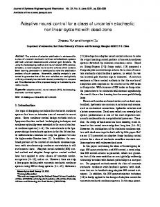
where α, c, and B1 are constants, c > 0 is the slope of lines satisfying c > B1 . Fig. 1 shows that the model (2) indeed generates a class of backlash-like hysteresis curve, where α = 1.0, c = 3.1635, B1 = 0.345 and the input signal v = 6.5 sin(2.3t). 20 15 10 5 u

0

The control objective is to design adaptive control law v(t) for system (5) such that the output y follows the specified desired trajectory yd . To facilitate the control design later in Section III, the following assumptions are needed. Assumption 1: The signs of gi are known, and there exist constants gi max ≥ gi min > 0 such that gi min ≤ |gi | ≤ gi max . Assumption 2: The desired trajectory vectors are continuous and available, and [yd , y˙ d , y¨d ]T ∈ Ωd with known compact set Ωd = {[yd , y˙ d , y¨d ]T : yd2 + y˙ d2 + y¨d2 ≤ B0 } ⊂ R3 , whose size B0 is a known positive constant. Assumption 3: [4] There exist constants cmin and cmax such that the slope c in (2) satisfies c ∈ [cmin , cmax ]. Assumption 4: [4] There exist a constant hmax such that h(v) ≤ hmax . Assumption 5: There exist constants di max such that di (t) ≤ di max . Remark 1: Assumption 1 implies that unknown constants gi are strictly either positive or negative. Without losing generality, we will only consider the case when gi > 0. Assumptions 3 and 4 assume the slop range of a backlash hysteresis and the upper bound of the hysteresis loop, which are reasonable according to the analysis in [4]. In Assumption 5, the disturbances are also required to be bounded, which is practical in reality. It should be noted that all these bounds gmax , gmin , cmin , cmax , hmax and di max are not required in implementation proposed control design. They are used only for analytical purposes.

−5

III. C ONTROL D ESIGN AND S TABILITY A NALYSIS

−10 −15 −20 −8

−6

−4

Fig. 1.

−2

0 v

2

4

6

8

Backlash-like Hystersis curve

Based on the analysis in [4], (2) can be solved explicitly as follows: u(t) = cv(t) + h(v)

(3)

where h(v) = [u0 − cv0 ]e−α(v−v0 )sgnv˙ Z v ˙ +e−αvsgnv˙ [B1 − c]eαζ(sgn v) dζ

(4)

v0

Substituting (3) into (1), we have: x˙ 1 x˙ i

x˙ n y

= .. . = ... = =

f1 (x1 ) + g1 x2 + d1 (t)

In this section, we will combine the dynamic surface control with backstepping and adaptive control for the nth-order system described by (5). Similar to traditional backstepping, the design of adaptive dynamic surface control is based on the following change of coordinates: z1 = x1 −yd , zi = xi − ωi , i = 2, ..., n, where ωi is the output of a first order filter with αi−1 as the input, and αi−1 is an intermediate control which shall be developed for the corresponding (i − 1)th subsystem. Finally, an overall control law v is constructed at step n. The major difference of dynamic surface control with traditional backstepping is to replace, at each step of recursion, the quantity α˙ i−1 by ω˙ i in determining the virtual control α˙ i . As a result, the operation of differentiation can be replaced by simpler algebraic operation. Before proceeding with the adaptive control, some notations are presented below: z¯i = [z1 , ..., zi ]T , y¯j = [y2 , ..., yj ]T , ¯ˆ ˆT ˆT T W i = [W1 , ..., Wi ] , where i = 1, ..., n, yj = ωj − αj−1 , j = 2, ..., n. Step 1: Since z1 = x1 − yd , and its derivative is z˙1

fi (¯ xi ) + gi xi+1 + di (t), i = 2, ..., n − 1

= x˙ 1 − y˙ d = f1 (x1 ) + g1 x2 + d1 (t) − y˙ d

(6)

Consider the following Lyapunov function candidate: fn (¯ xn ) + gn cv(t) + gn h(v) + dn (t) x1

(5)

4483

Vz1

=

1 2 z 2g1 1

(7)

Its derivative along (6) is V˙ z1

Substituting (17) and (18) into (16) leads to

1 z1 z˙1 g1

=

= z1 [Q1 (Z1 ) + x2 +

1 d1 (t)] g1

(8)

where Q1 (Z1 ) = g1−1 f1 (x1 ) − g1−1 y˙ d with Z1 = [x1 , y˙ d ] ∈ ΩZ1 ⊂ R2 . To compensate for the unknown function Q1 (Z1 ), we can use the radial basis function neural network ˆ 1 ∈ Rl×1 , S(Z1 ) ∈ ˆ T S(Z1 ), with W (RBFNN) in [11], W 1 l×1 R , and the NN node number l > 1, to approximate the function Q1 (Z1 ) on the compact set ΩZ1 as follows ˆ 1T S(Z1 ) − W ˜ 1T S(Z1 ) + ε1 (Z1 ) Q1 (Z1 ) = W

(9)

where the approximation error ε1 (Z1 ) satisfies |ε1 (Z1 )| ≤ ε∗1 with a positive constant ε∗1 . Substituting (9) into (8) and according to Assumptions 1 and 5, we obtain V˙ z1

ˆ 1T S(Z1 ) − W ˜ 1T S(Z1 ) + x2 ] + |z1 |D1(10) z1 [W

≤

where D1 = becomes V˙ z1

d1max g1 min

1 1 ˜ 1T S(Z1 ) −(k1 − 2)z12 + z22 + y22 − z1 W 4 4 z1 ˜ (19) −z1 tanh( )D 1 + 0.2785ǫD1 ǫ Define the filtered virtual control ω2 in the following manner: V˙ z1

+ ε∗1 . Since x2 = z2 + y2 + α1 , (10)

˜ 1T S(Z1 ) + z2 + y2 + α1 ] ˆ 1T S(Z1 ) − W ≤ z1 [W +|z1 |D1 (11)

τ2 ω˙ 2 + ω2 = α1 ,

ˆ˙ 1 W ˆ˙ 1 D

ˆ 1T S(Z1 ) − tanh( z1 )D ˆ1 = −k1 z1 − W ǫ ˆ 1] = Γ1 [z1 S(Z1 ) − σ1 W z1 ˆ 1] = γd1 [z1 tanh( ) − σd1 D ǫ

(12)

= ω˙ 2 − α˙ 1 = −

As such, y2 ˆ 1, D ˆ 1 , yd , y˙ d , y¨d ) z2 , y2 , W y˙ 2 + ≤ ζ2 (¯ τ2

(22)

y2 1 y22 + |y2 |ζ2 ≤ − 2 + y22 + ζ22 τ2 τ2 4

(23)

ˆ 1, D ˆ 1 , yd , y˙ d , y¨d ) is a continuous function. where ζ2 (¯ z2 , y2 , W From (21) and (22), using the Young’s inequality, we obtain that y2 y˙ 2 ≤ −

Consider the following Lyapunov function candidate: V1

z1 ) ≤ 0.2785ǫ ǫ

V˙ 1

(15)

we obtain that V˙ z1

˜ 1T S(Z1 ) −k1 z12 + z1 z2 + z1 y2 − z1 W z1 ˆ −z1 tanh( )D1 + |z1 |D1 ǫ ˜ 1T S(Z1 ) ≤ −k1 z12 + z1 z2 + z1 y2 − z1 W z1 z1 ˜ −z1 tanh( )D1 + |z1 |D1 − z1 tanh( )D1 ǫ ǫ ˜ 1T S(Z1 ) ≤ −k1 z12 + z1 z2 + z1 y2 − z1 W z1 ˜ (16) −z1 tanh( )D 1 + 0.2785ǫD1 ǫ

≤

˜ = D ˆ − D. Using the Young’s inequality, the where D following inequalities hold: z1 z2 z1 y2

1 ≤ z12 + z22 4 1 2 ≤ z1 + y22 4

(17)

1 ˜2 1 2 1 ˜ T −1 ˜ D + y (24) = Vz 1 + W 1 Γ1 W 1 + 2 2γd1 1 2 2

Its time derivative along (19) and (23) is

ˆ 1 is the estimate of D1 , Γ1 = ΓT ∈ where k1 > 0, ǫ > 0, D 1 l×l R > 0, σ1 > 0, γd1 > 0 and σd1 > 0. Substituting (12) into (11), and using the following property of the hyperbolic tangent function tanh(·): 0 ≤ |z1 | − z1 tanh(

(20)

T y2 ˆ˙ 1 S(Z1 ) + W ˆ 1T S(Z ˙ 1) + [k1 z˙1 + W τ2 z1 ˆ˙ 2 z1 ˆ 1] + tanh( )D ))z˙1 D (21) 1 + (1 − tanh ( ǫ ǫ

y˙ 2

(13) (14)

ω2 (0) = α1 (0),

where τ2 is a design constant that we will choose later. Due to y2 = ω2 − α1 , from (20), we have ω˙ 2 = − yτ22 . Therefore, we have

Choose the following virtual control law and adaptation laws: α1

≤

˜˙ 1 + 1 D ˜ 1T Γ−1 W ˜D ˜˙ + y2 y˙ 2 = V˙ z1 + W 1 γd1 1 ˜ T S(Z1 ) ≤ −(k1 − 2)z12 + z22 − z1 W 1 4 z1 ˜ ˜ 1T Γ−1 W ˆ˙ 1 −z1 tanh( )D1 + 0.2785ǫD1 + W 1 ǫ 1 ˜ ˆ˙ 1 1 y2 + (25) DD − 2 + 1 y22 + ζ22 γd1 τ2 4 4

Substituting (13) and (14) into (25) results in V˙ 1

≤

1 ˆ1 ˜ 1D ˆ 1 − σd D ˜ 1T W −(k1 − 2)z12 + z22 − σ1 W 1 4 y2 1 1 − 2 + 1 y22 + ζ22 + 0.2785ǫD1 (26) τ2 4 4

Step i (2 ≤ i < n): The time derivative of zi is z˙i = fi (¯ xi ) + gi xi+1 + di (t) − ω˙ i

(27)

Consider the following Lyapunov function candidate: Vzi

=

1 2 z 2gi i

(28)

Its derivative along (27) is

(18)

4484

V˙ zi

=

1 1 zi z˙i = zi [Qi (Zi ) + xi+1 + di (t)] (29) gi gi

where Qi (Zi ) = gi−1 fi (¯ xi ) − gi−1 ω˙ i with Zi = [¯ xi , ω˙ i ] ∈ i+1 ΩZi ⊂ R . To compensate for the unknown function Qi (Zi ), we can use the radial basis function neural network ˆ T S(Zi ), with W ˆ i ∈ Rl×1 , S(Zi ) ∈ Rl×1 , and (RBFNN), W i the NN node number l > 1, to approximate the function Qi (Zi ) on the compact set ΩZi as follows ˆ iT S(Zi ) − W ˜ iT S(Zi ) + εi (Zi ) Qi (Zi ) = W

(30)

where the approximation error εi (Zi ) satisfies |εi (Zi )| ≤ ε∗i with a positive constant ε∗i . Substituting (30) into (29), we obtain ˜ iT S(Zi ) + xi+1 ] + |zi |Di ˆ iT S(Zi ) − W ≤ z i [W (31)

V˙ zi

+ ε∗i . Since xi+1 = zi+1 + yi+1 + αi , where Di = dg11 max min (31) becomes V˙ zi

ˆ iT S(Zi ) − W ˜ iT S(Zi ) + zi+1 + yi+1 + αi ] ≤ zi [W +|zi |Di

(32)

Choose the following virtual control law and adaptation laws: ˆi ˆ iT S(Zi ) − tanh( zi )D (33) αi = −ki zi − W ǫ ˆ i] ˆ˙ i = Γi [zi S(Zi ) − σi W (34) W zi ˙ˆ ˆ i] (35) Di = γdi [zi tanh( ) − σdi D ǫ ˆ i is the estimate of Di , Γi = ΓT ∈ where ki > 0, ǫ > 0, D i l×l R > 0, σi > 0, γdi > 0 and σdi > 0. Substituting (33) into (32) and using the property of the hyperbolic tangent function as (15), we obtain V˙ zi

˜ T S(Zi ) −ki zi2 + zi zi+1 + zi yi+1 − zi W i zi ˜ (36) −zi tanh( )Di + 0.2785ǫDi ǫ Using the Young’s inequality, the following inequalities hold: 1 2 zi zi+1 ≤ zi2 + zi+1 (37) 4 1 2 (38) zi yi+1 ≤ zi2 + yi+1 4 Substituting (37) and (38) into (36) leads to 1 2 1 2 ˜ iT S(Zi ) + yi+1 − zi W V˙ zi ≤ −(ki − 2)zi2 + zi+1 4 4 zi ˜ (39) −zi tanh( )D i + 0.2785ǫDi ǫ Define the filtered virtual control ωi+1 in the following manner: ≤

τi+1 ω˙ i+1 + ωi+1 = αi ,

ωi+1 (0) = αi (0),

(40)

where τi+1 is a design constant that we will choose later. Due to yi+1 = ωi+1 − αi , from (40), we have ω˙ i+1 = i+1 − yτi+1 . Therefore, we have y˙ i+1

= ω˙ i+1 − α˙ i T yi+1 ˆ˙ i S(Zi ) + W ˆ iT S(Z ˙ i) + [ki z˙i + W = − τi+1 zi ˆ˙ 2 zi ˆ + tanh( )D i + (1 − tanh ( ))z˙i Di ] (41) ǫ ǫ

As such, yi+1 ¯ˆ ¯ˆ zi+1 , y¯i+1 , W ¨d ) (42) ≤ ζi+1 (¯ y˙ i+1 + i , D i , yd , y˙ d , y τi+1 ¯ˆ ¯ˆ where ζi+1 (¯ zi+1 , y¯i+1 , W ¨d ) is a continuous i , D i , yd , y˙ d , y function. From (41) and (42), using the Young’s inequality, we obtain that y2 y2 2 yi+1 y˙ i+1 ≤ − i+1 + |yi+1 |ζi+1 ≤ − i+1 + yi+1 τi+1 τi+1 1 2 (43) + ζi+1 4 Consider the following Lyapunov function candidate: 1 ˜ T −1 ˜ 1 ˜2 1 2 Vi = Vzi + W Γ Wi + D + yi+1 (44) 2 i i 2γdi i 2 Its time derivative along (39) and (43) is ˜D ˜˙ i + yi+1 y˙ i+1 ˜˙ i + 1 D ˜ iT Γ−1 W V˙ i = V˙ zi + W i γdi 1 2 ˆ˙ i ˜ iT Γ−1 W ˜ iT S(Zi ) + W ≤ −(ki − 2)zi2 + zi+1 − zi W i 4 y2 1 2 1 2 1 ˜ ˆ˙ + ζi+1 (45) DDi − i+1 + 1 yi+1 + γdi τi+1 4 4 Substituting (34) and (35) into (45) results in 1 2 ˜ iD ˆi ˜ TW ˆ i − σd D V˙ i ≤ −(ki − 2)zi2 + zi+1 − σi W i i 4 y2 1 2 1 2 + ζi+1 + 0.2785ǫDi (46) − i+1 + 1 yi+1 τi+1 4 4 Step n: In this final step, we will design the control input v(t). Since zn = xn − ωn , the time derivative of zn is z˙n = fn (¯ xn ) + gn cv(t) + gn h(v) + dn (t) − ω˙ n Consider the following Lyapunov function candidate: 1 2 z Vzn = 2gn c n Its derivative along (47) is V˙ zn

=

(47)

(48)

h(v) 1 zn z˙n = zn [Qi (Zn ) + v(t) + gn c c 1 + dn (t)] (49) gn c

where Qn (Zn ) = (gn c)−1 fn (¯ xn ) − (gn c)−1 ω˙ n with Zn = n+1 [¯ xn , ω˙ n ] ∈ ΩZn i ⊂ R . To compensate for the unknown function Qn (Zn ), we can use the radial basis function neural ˆ nT S(Zn ), with W ˆ n ∈ Rl×1 , S(Zn ) ∈ network (RBFNN), W l×1 R , and the NN node number l > 1, to approximate the function Qn (Zn ) on the compact set ΩZn as follows ˆ nT S(Zn ) − W ˜ nT S(Zn ) + εn (Zn ) Qn (Zn ) = W

(50)

where the approximation error εn (Zn ) satisfies |εn (Zn )| ≤ ε∗n with a positive constant ε∗n . Substituting (50) into (53)and according to Assumptions 1, 3-5, we obtain that

4485

V˙ zn

≤

˜ nT S(Zn ) + v(t)] + |zn |Dn ˆ nT S(Zn ) − W zn [W (51)

where Dn = control law:

hmax cmin

+

dn max gn min cmin

+ ε∗n . Choose the following

Substitute (26)(46) and (58) into (59), it follows that V˙

ˆ nT S(Zn ) − tanh( zn )D ˆn = −kn zn − W ǫ

v(t)

≤ −(k1 − 2)z12 −

(52)

−

ˆ n is the estimate of Dn . Substituting where kn > 0, ǫ > 0, D (52) into (51), and using the property of the hyperbolic tangent function as (15), we obtain that V˙ zn

˜ nT S(Zn ) − zn tanh( zn )D ˜n ≤ −kn zn2 − zn W ǫ +0.2785ǫDn (53)

˜n = D ˆ n − Dn . where D Consider the following Lyapunov function candidate: Vn

1 ˜2 1 ˜ T −1 ˜ Γ Wn + D = Vzn + W 2 n n 2γdn n

(54)

where Γn = ΓTn ∈ Rl×l > 0, γdn > 0. Its time derivative along (53) is V˙ n

= ≤

1 ˜ ˜˙ ˜ nT Γ−1 ˜˙ Dn D n V˙ zn + W n Wn + γdn ˜ nT S(Zn ) − zn tanh( zn )D ˜n −kn zn2 − zn W ǫ 1 ˜ ˆ˙ ˆ˙ ˜ nT Γ−1 +0.2785ǫDn + W Dn Dn (55) n Wn + γdn

ˆ n] = Γn [zn S(Zn ) − σn W zn ˆ n] = γdn [zn tanh( ) − σdn D ǫ

(56)

1 1 (ki − 2 )zi2 − (kn − )zn2 4 4 i=2

˜ TW ˆi − σi W i

n X

˜ iD ˆi + σdi D

n−1 Xh i=1

i=1

i=1

−

2 yi+1 τi+1

n 1 2 i X 1 2 + ζi+1 0.2785ǫDi + +1 yi+1 4 4 i=1

(60)

Since for any B0 > 0 and p > 0, the sets Ωd = {(yd , y˙ d , y¨d ) : ¯ˆ T T Pi Vj ≤ y 2 + y˙ 2 + y¨2 ≤ B0 } and Ωi = {[¯ z T , y¯T , W i ] : d

d

i

d

i

j=1 Pi

p}, i = 1, ..., n are compact in R3 and R2i−1+ j=1 lj , respectively. Therefore, ζi+1 has a maximum Mi+1 on Ωd × Ωi . By completion of squares, the following inequalities hold: ∗ 2 ˜ 2 ˜ TW ˆ i ≤ − σi kWi k + σi kWi k −σi W (61) i 2 2 2 ˜2 ˆ i ≤ − σdi Di + σdi Di ˜ iD (62) −σdi D 2 2 Substituting (61) and (62) into (60) leads to V˙

≤

−(k1 − 2)z12 − −

n−1 X

1 1 (ki − 2 )zi2 − (kn − )zn2 4 4 i=2

n X ˜ i k2 σi kW

−

2 i 1 2 +1 yi+1 +µ 4 i=1

Choose the following adaptation laws: ˆ˙ n W ˆ˙ n D

n X

n−1 X

n 2 X X h yi+1 ˜ 2 n−1 σdi D i − + 2 τi+1 i=1 i=1

(63)

where

(57)

µ =

n X σi kW ∗ k2 i

i=1

where σn > 0 and σdn > 0. Substituting (56) and (57) into (55) results in

+

n X

2

+

n n−1 X σdi Di2 1X 2 + M 2 4 i=1 i+1 i=1

0.2785ǫDi

(64)

i=1

V˙ n

≤

ˆ n + 0.2785ǫDn ˜ nD ˜ nT W ˆ n − σd D −kn zn2 − σn W n (58)

The following theorem shows the stability and control performance of the closed-loop adaptive system. Theorem 1: Consider the closed-loop system consisting of the plant (5) under Assumptions 1-5, the controller (52), and adaption laws (34)(35). For bounded initial conditions, there exist constants p > 0, ki > 0, τiP> 0, λmax (Γ−1 i ), σi > 0, n γdi and σdi > 0, satisfying V = i=1 Vi ≤ p, such that the overall closed-loop control system is semi-globally stable in the sense that all of the signals in the closed-loop system are bounded, and the tracking error is smaller than a prescribed error bound. Consider the Lyapunov function candidate V = PProof: n i=1 Vi . Its derivative with respect to time is: V˙ =

n X i=1

V˙ i

(59)

Choosing α0

≤ min{σdi γdi ,

σi }, i = 1, ..., n λmax (Γ−1 i )

α0 2g1 min α0 1 , i = 2, ..., n − 1 ki ≥ 2 + 4 2gi min 1 α0 kn ≥ + 4 2gi min cmin 1 1 α0 ≥ 1 + , i = 2, ..., n τi 4 2 and substituting them into (60), we obtain that k1

≥ 2+

V˙ ≤ −α0 V + µ

(65)

(66)

then V˙ ≤ 0. If implies that V (t) ≤ If V = p and α0 > p, ∀t ≥ 0 for V (0) ≤ p. Multiplying (66) by eα0 t and integrating over [0, t] yields h µ i −α0 t µ + V (0) − e (67) 0 ≤ V (t) ≤ α0 α0

4486

µ p,

IV. S IMULATION S TUDIES To demonstrate the effectiveness of the proposed approach, we consider the plant used in [4] and [5]: x˙ = a y

1 − e−x(t) + bu(v) 1 + e−x(t)

= x

(68)

where a = 1, b = 1, and u(v) represents an output of the following backlash-like hysteresis: dv du dv = α (cv − u) + B1 (69) dt dt dt

[4] C. Y. Su, Y. Stepanenko, J. Svoboda, and T. P. Leung, “Robust adaptive control of a class of nonlinear systems with unknown backlash-like hysteresis,” IEEE Transactions on Automatic Control, vol. 45, no. 12, pp. 2427–2432, 2000. [5] J. Zhou, C. Y. Wen, and Y. Zhang, “Adaptive backstepping control design of a class of uncertain nonlinear systems with unknown backlash-like hysteresis,” IEEE Transactions on Automatic Control, vol. 49, no. 10, pp. 1751–1757, 2004. [6] S. S. Ge, C. C. Hang, T. H. Lee, and T. Zhang, Stable Adaptive Neural Network Control. Boston: Kluwer Academic Publisher, 2002. [7] J. A. Farrell and M. M. Polycarpou, Adaptive Approximation Based Control. Hoboken, NJ: Wiley, 2006. [8] F. L. Lewis, S. Jagannathan, and A. Yesilidrek, Neural Network Control of Robot Manipulators and Nonlinear Systems. Philadelphia, PA: Taylor and Francis, 1999. [9] D. Swaroop, J. K. Hedrick, P. P. Yip, and J. C. Gerdes, “Dynamic surfance control for a class of nonlinear systems,” IEEE Transactions on Automatic Control, vol. 45, no. 10, pp. 1893–1899, 2000. [10] D. Wang and J. Huang, “Neual network-based adaptive dynamic surface control for a class of uncertain nonliear systems in strictfeedback form,” IEEE Transactions on Neural Netowrks, vol. 16, no. 1, pp. 195–202, 2005. [11] R. M. Sanner and J. E. Slotine, “Gaussian networks for direct adaptive control,” IEEE Transactions on Neural Networks, vol. 3, no. 6, pp. 837–863, 1992.

with α = 1, c = 3.1635, and B1 = 0.345. As discussed in [4], without control, i.e., u(v) = 0, (68) is unstable, since −x(t) −x(t) x˙ = a 1−e > 0 for x > 0, and x˙ = a 1−e < 0 for 1+e−x(t) 1+e−x(t) x < 0. The objective is to control the system output y to follow a desired trajectory yd = 12.5 sin(2.3t). We adopt the control law and adaption laws in (52) (56) (57). The following initial conditions and control design parameters are chosen as: x(0) = u(0) = v(0) = 0.0, ˆ (0) = D(0) ˆ W = 0.0, k1 = 0.3, Γ = 0.1I25 , σ = 0.1, γd = 0.1,σd = 0.1, ǫ = 0.05. The simulation results are shown in Figs. 2 and 3. From Fig. 2, we observe that good tracking performance is achieved and the tracking error converges to a small neighborhood of zero. At the same time, the control signal v and hysteresis output u are kept bounded, as seen in Figs. 3. It is noted that there is a large difference between the signals v and u in Fig. 3, which indicates the significant hysteresis effect.

15 y y

10

Tracking performance

Therefore, all signals of the closed-loop system, i.e., zi , yi ˆ i are uniformly ultimately bounded. Furthermore, and W xi , αi and Ωi are also uniformly ultimately bounded. From (64) and (65), we know that for any given constants B0 , p, σdi and σi , we can decrease λmax (Γ−1 i ) to make µ arbitrarily small. Thus, the tracking error z1 becomes α0 arbitrarily small. This completes the proof.

d

5

0

−5

−10

−15

0

5

Fig. 2.

10 Time [s]

15

20

Tracking performance

V. C ONCLUSION 30 u

20

10 Control singals

Adaptive dynamic surface control (DSC) using neural networks has been proposed for a class of nonlinear systems in strict-feedback form with back-lash hysteresis input, where the hysteresis is modeled as a differential equation. The developed adaptive control can guarantee that all signals involved are semi-globally uniformly ultimately bounded (SGUUB) without constructing a hysteresis inverse. Simulation results have been provided to show the effectiveness of the proposed approach.

v 0

−10

R EFERENCES [1] G. Tao and P. V. Kokotovic, “Adaptive control of plants with unknown hysteresis,” IEEE Transactions on Automatic Control, vol. 40, pp. 200– 212, 1995. [2] J. W. Macki, P. Nistri, and P. Zecca, “Mathematical models for hysteresis,” SIAM Review, vol. 35, pp. 94–123, 1993. [3] X. Tan and J. S. Baras, “Modeling and control of hysteresis in magnestrictive actuators,” Automatica, vol. 40, no. 9, pp. 1469–1480, 2004.

4487

−20

−30

0

5

Fig. 3.

10 Time [s]

Control inputs

15

20