Adaptive Filtering of Heart Rate Signals for an Improved ... - CiteSeerX

INTERNATIONAL JOURNAL OF SIGNAL PROCESSING VOLUME 2 NUMBER 1 2005 ISSN 1304-4478

Adaptive Filtering of Heart Rate Signals for an Improved Measure of Cardiac Autonomic Control Desmond B. Keenan, Paul Grossman high-frequency band (HF), loosely defined between 0.15 and 0.4 Hz and known as respiratory sinus arrhythmia (RSA) because it occurs at the respiratory frequency. The magnitude of this high frequency band has been demonstrated to be associated with the extent of cardiac parasympathetic activity in pharmacological autonomic blockade studies [2] respiratory sinus arrhythmia, cardiac vagal tone, and respiration: withinand between-individual relations. The ratio of power in the LF and HF components (LF/HF) has been used to provide an estimate of cardiac sympathovagal balance, although this measure remains in dispute [3]. Nevertheless, several studies have indicated that when considered jointly, HF and LF HRV may provide useful information about both sympathetic and parasympathetic influences upon the cardiac cycle [4-6]. A correlation between body fat content and the LF/HF ratio after glucose ingestion have been correlated in nonobese subjects with various levels of body fat content [7]. Decreased values of HRV are indirectly proportional to pressure, body mass index and insulinemia in young and obese patients without clinical symptoms of cardiovascular disease, diabetes or damage of target organs [8]. These HRV measurements can also be sensitive to stress and can be seen to decrease with age, which has been attributed to a decrease in efferent vagal tone. On the other hand, regular exercise has been shown to increase vagal tone. Measures of mortality have been examined primarily with patients who have undergone cardiac surgery. Clinical depression strongly associated with mortality with such patients is often associated with a decrease in HRV [9]. Spectral HRV was previously described as a measure of power in various frequency bands. To determine the RSA amplitude over a period of time, frequency domain, time domain and phase domain approaches have been analyzed [10]. A time-domain approach by Grossman [10] known as the peak-valley algorithm measures the maxima and minima values of R-to-R time intervals within each breath. In the frequency domain a value for RSA can be derived by applying an appropriate window function to a given time series to reduce spectral leakage from random events and applying the Fourier transform to the filter residuals. When analyzing the HF band the respiratory frequency should be predetermined through some kind of respiratory sensor, determined through paced breathing or at the very least estimated by means of

Abstract—In order to provide accurate heart rate variability indices of sympathetic and parasympathetic activity, the low frequency and high frequency components of an RR heart rate signal must be adequately separated. This is not always possible by just applying spectral analysis, as power from the high and low frequency components often leak into their adjacent bands. Furthermore, without the respiratory spectra it is not obvious that the low frequency component is not another respiratory component, which can appear in the lower band. This paper describes an adaptive filter, which aids the separation of the low frequency sympathetic and high frequency parasympathetic components from an ECG R-R interval signal, enabling the attainment of more accurate heart rate variability measures. The algorithm is applied to simulated signals and heart rate and respiratory signals acquired from an ambulatory monitor incorporating single lead ECG and inductive plethysmography sensors embedded in a garment. The results show an improvement over standard heart rate variability spectral measurements.

Keywords—Heart rate variability, vagal tone, sympathetic, parasympathetic, spectral analysis, adaptive filter.

H

I. INTRODUCTION

EART rate variability (HRV) is a measure of alterations in heart rate derived by measuring the variation of RR intervals, and HRV parameters have been shown to aid assessment of cardiovascular disease [1]. Heart rate is influenced by both sympathetic and parasympathetic (vagal) activity. The influence and balance of both branches of the autonomic nervous system (ANS) have been termed sympathovagal balance and is reflected in the RR interval changes. HRV is frequently estimated by means of spectral analysis in which power in three or four frequency bands is determined. A low frequency (LF) component has been proposed as reflecting both sympathetic and parasympathetic effects on the heart and generally occurs in a band between 0.04 Hz and 0.15 Hz. Chemoreceptor processes, thermoregulation, and the rennin-angiotensin system have been tied to very low frequencies. The influence of vagal efferent modulation of the sinoatrial node can be seen in the D. B. Keenan is with Research and Development, Medtronic MiniMed, Northridge, CA 91325 USA (phone: 818-576-4472; fax: 818-576-6206; email: barry.keenan@ medtronic.com). P. Grossman is with the Department of Psychosomatic & Internal Medicine University of Basel Hospital, Petersgraben 4, CH-4031 Basel, Switzerland (email: [email protected]).

IJSP VOLUME 2 NUMBER 1 2005 ISSN 1304-4478

52

© 2005 INTERNATIONAL ACADEMY OF SCIENCES

INTERNATIONAL JOURNAL OF SIGNAL PROCESSING VOLUME 2 NUMBER 1 2005 ISSN 1304-4478

contribution of each band to overall tidal volume based on Equation (1)

dominant frequencies. The frequency domain approach takes the average response over time, e.g. a 5-minute period or longer. This approach provides little information about the RSA waveform as it is time averaged and may not reflect cardiac vagal dynamics. Another approach to evaluating RSA has been to analyze dynamics of the heart rate with respect to respiratory phase [11] known as the phase domain approach. Waveforms in the phase-domain were shown to be similar regardless of breathing pattern. By looking at heart rate with respect to phase showed synchronous patterns during paced breathing and useful to extract RSA during spontaneous breathing. One preprocessing approach by Korhonen et, al. [12] used multistage linear filtering methods as a ventilation cancellation filter to attenuate the effects of spontaneous respiration. This approach estimated slow baseline variations in the RR signal, which was linearly subtracted from the RR signal prior to analysis. Other investigations [13][14] describe a time-domain decomposition to assess vagal tone. This methodology uses an adaptive filter to separate the respiratory influence from the nonrespiratory sympathetic variations to measure the magnitude of the RSA component. Presented in this paper is an adaptive filter, which can separate the LF and HF components and therefore acquire separate spectral analysis measures. This enables a uniformly sampled RSA waveform to be linearly predicted which more accurately reflects cardiac vagal dynamics in the time-domain. With time-domain LF and HF signals more accurate statistical measures can be applied. II.

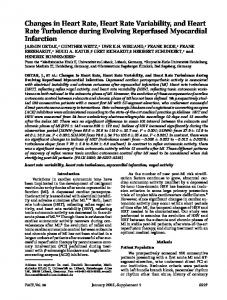
where Vt is the tidal volume measurement, RC and AB are the ribcage and abdominal bands, and k and l are calibration coefficients that apply the appropriate gain to each signal based on a calibration algorithm [20][21]. The LifeShirt also contains a single lead ECG sampled at 200 Hz, which is linearly interpolated to 1 kHz, and heart rate is determined based on R wave locations determined from Pan and Tomkins QRS detection algorithm [22]. B. Spectral Analysis The derived RR intervals are preprocessed prior to spectral analysis. This process is illustrated in Figure 1 where the instantaneous RR intervals are uniformly sampled at 50Hz and downsampled to 5Hz. RR

|H(jω)|

RR ∆t = 20msec

LPF Fc = 2.5 Hz

RR ∆t = 0.2sec

Linear Figure Detrend 14

RR = RR – mean(RR)

Buffer t = 5 mins

Fig. 1 Block diagram of HRV preprocessing

METHODS

Five-minute time windows are detrended using a best straight line fit approach with the segment mean removed. Welch's [23] power spectral density estimation approach is then applied. Welch's averaged, modified periodogram method applies sections of the RR signal with 50% overlap, with each section windowed with a Hamming window and nine modified periodograms are computed and averaged. A five-minute window is decomposed into 1-minute windows with 300 samples; sampled at 5 Hz. Each 1 minute window is zero padded to a 2048 sample length and the power of the FFT averaged. Various window functions may be applied, although a rectangular window will normally introduce some spectral leakage, and other window functions such as Blackman-Harris and Nutal can smear the spectra, but are also preferred in certain circumstances. The power in the LF and HF bands are then calculated across their given ranges 0.040.15 and 0.14-0.4 Hz respectively [24].

A. Data Collection The data in this investigation was collected from the LifeShirt. The LifeShirt employs the Konno and Mead [15] two compartment-breathing model of the respiratory system. This approach shows changes in tidal volume measured at the mouth to be comparable to the sum of changes in ribcage and abdominal contributions. These volume changes are normally obtained by measuring variations in the thoracic and abdominal regions by inductive plethysmography (IP), magnetometers, or strain gauges [16-18]. The LifeShirt contains two IP sensors encircling the ribcage and abdomen used to measure tidal volume. Studies comparing IP with pneumotachographic airflow measurements have reported correlation accuracies of r=0.96 and greater [19]. To measure the self-inductance of these IP sensors a low oscillating current is passed through the inductive bands creating a magnetic field. The self-inductance of the coil is proportional to the cross sectional area of the band. As this cross sectional area changes the coils self-inductance changes. Changes in self-inductance are measured by integrating an oscillator circuit whose resonant frequency varies with changes in selfinductance. A counter measures this resonant frequency by counting the pulses produced by the oscillator over time, creating a waveform proportional to changes in the cross sectional area. The IP bands are calibrated to apply the correct

IJSP VOLUME 2 NUMBER 1 2005 ISSN 1304-4478

(1)

Vt = k.RC + l. AB

C. Adaptive Filtering Prior to spectral analysis the RR and Vt signals are fed into an LMS adaptive filter in order to separate the LF and HF components. The least mean square (LMS) adaptive filter algorithm [25] requires tuning a set of FIR filter coefficients to model the difference between the input RR signal and the reference signal Vt. The LMS algorithm computes a set of optimum coefficients, which are adjusted to minimize the mean squared error (MSE) between the two signals. This

53

© 2005 INTERNATIONAL ACADEMY OF SCIENCES

INTERNATIONAL JOURNAL OF SIGNAL PROCESSING VOLUME 2 NUMBER 1 2005 ISSN 1304-4478

algorithm is based on the steepest decent algorithm where the weights are updated on a sample-by-sample basis described by (4). This is a practical approach to obtaining estimates of the filter weights w in real-time without having to perform any type of matrix inversions which require a lot more computation. The algorithm doesn’t require prior statistical knowledge of the signal and instead uses instantaneous estimates. Therefore, the weights obtained by the LMS algorithm are estimates that gradually improve over time as the filter weights are adjusted as the filter learns the characteristics of the signal, and eventually converge. Figure 2 best describes this algorithm where both signals are downsampled to the same rate. RR

LPF

+

↓10

-

Vt

Σ

D. Simulation Design Before applying the adaptive filter to real signals a simulation was designed to be roughly representative of the characteristics of real life respiratory and heart rate signals. This enables simple testing of the filter’s characteristics and performance and facilitates approximations of the filters parameters. Equations (5) and (6) express the simulated RR interval signals and tidal volume signals respectively, (5)

Vt (t ) = D cos(2πf h t ) + E

(6)

where A is the peak-to-peak RSA amplitude per breath expressed in msec, B is the LF/HF ratio expressed as a fraction of A and C is the mean RR interval. Tidal volume is expressed by D, and E is a DC offset whose values depends on ribcage and abdominal cross sectional area, which varies with changes in posture and mass, as the respiratory signals are DC coupled. The parasympathetic (HF) component and sympathetic (LF) component have frequencies fh , fl and phases αh, αl respectively. The signals are sampled with 1msec resolution where t = 0, 0.001..299, for a 300 second or 5 minute duration. The instantaneous RR interval signal is thus derived from Equations (7) and (8) where the sum of all previous RR intervals determines the time of the beat that is applied to Equation (9), where i is the beat number.

z

y ↓10

s(t ) = A sin(2πf h t + α h ) + B sin(2πf l t + α l ) + C

Adaptive Filter

Fig. 2 LMS Adaptive filter

A set of weights is first initialized to zero. For each subsequent sampling instants k the filter output is computed using an FIR filter structure expressed by Equation (2) where the output y is the filtered tidal volume (Vt) signal predicting the respiratory or RSA component in the RR interval signal.

RR(0) = s(0) = C

(7)

⎞ ⎛ RR(i) = s⎜1000∑ RR(n) ⎟ n =0 ⎠ ⎝

(8)

i −1

N −1

y k = ∑ wiVt k −i

(2)

i =0

Each sample is then repeated for the duration of the cycle length in 20msec sample intervals providing the 50 Hz sample rate expressed as follows:

Having predicted this signal y it is now possible to linearly subtract that component. The Vt signal is decimated by a factor of 10; downsampled to 5 Hz and the RR interval signal is resampled at 5 Hz to synchronize the samples of each signal. The RR interval signal is derived from a 1 lead ECG applying the Pan-Tomkins algorithm [22]. This signal is sampled at a rate of 50 Hz and low-pass filtered before decimating by 10 to produce a 5 Hz signal. The filter of length N is normally chosen dependant on the amount of memory required for the filter. The error estimate in this structure is the algorithm output and is computed as z k = RRk − y k

RRcont (k ) = RR(i),

IJSP VOLUME 2 NUMBER 1 2005 ISSN 1304-4478

(9)

This procedure emulates the data acquisition procedure for acquiring the continuous RR signal. By acquiring samples at a uniform rate (50 Hz) the signal can be uniformly decimated to 5 Hz. III. RESULTS The following investigations use the simulation previously described with selected parameters in order to first test the accuracy of the filter. Real signals are later applied using data collected from LifeShirt. The output of the first simulation (simulation A) is illustrated in Figure 3 for one parameter set with high and low frequencies of 0.2 and 0.1 Hz respectively. No phase variation was applied to this signal. An RSA amplitude of A = 200 msec was used with B =100 to give a 50% LF/HF ratio. These signals were applied to the adaptive

(3)

where z is the LF component and y is the predicted HF or RSA component. The filter weights w are updated based on this error expressed in Equation (4), where µ controls the rate of convergence and the stability of the filter. On each iteration of the LMS adaptive algorithm, the MSE is minimized. wi = wi + 2µzkVti −1

k = i,0.02....i + 1

(4)

54

© 2005 INTERNATIONAL ACADEMY OF SCIENCES

INTERNATIONAL JOURNAL OF SIGNAL PROCESSING VOLUME 2 NUMBER 1 2005 ISSN 1304-4478

Fig. 4 Adaptive filter outputs for Simulation A

Fig. 3 Simulation A. Vt and RR signals

Fig. 6 Simulation B. Vt and RR signals

Fig. 5 HRV spectra for simulation A

Fig. 8 HRV spectra for simulation B

Fig. 7 Adaptive filter outputs for Simulation B

evident that the components are accurately decomposed where the power in the HF and LF signal’s spectra is 2165ms2 (186 ms peak-to-peak) and 620ms2 (99.67 ms peak-to-peak) respectively. To adequately test the adaptive filter another set of signals were simulated (simulation B), where power leaked from the LF band into the adjacent HF band. The same parameters were and the HF component remaining at 0.2 Hz. The signals are illustrated in Figure 6. The first trace in Figure 6 is tidal volume (Vt), with a respiration rate of 5 seconds per breath or 0.2 Hz. This is representative of the typical average breath rate. The RR signal is downsampled via the preprocessing algorithm of Figure 1. The third trace of

the power in the HF and LF signal’s spectra is filter previously described with outputs shown in Figure 4. The second trace of Figure 4 shows the predicted HF component within the RR signal, predicted based of the reference signal Vt. It is evident from this trace that it took approximately 100 seconds for the filter to tune and adapt to simulation A’s characteristics. The LF signal is derived by linearly subtracting the HF signal from the original raw signal. HRV analysis is performed on the original signal and the 2 decomposed signals separately, applying the spectral routine of section 2.1 with the results illustrated in Figure 5. It is

IJSP VOLUME 2 NUMBER 1 2005 ISSN 1304-4478

55

© 2005 INTERNATIONAL ACADEMY OF SCIENCES

INTERNATIONAL JOURNAL OF SIGNAL PROCESSING VOLUME 2 NUMBER 1 2005 ISSN 1304-4478

Fig. 9 Filter output for example 1

Fig 10 Power spectra for example 1

Fig. 11 Filter output for example 2

Fig. 12 Power spectra for example 2

Fig. 13 Filter output for example 3

Fig. 14 Power spectra for example 3

only one component where the LF component smeared with have been accurately decomposed. The spectra is nearly a perfect match to that of Figure 5, where the power in the HF and LF signal’s spectra is 2106ms2 (183 ms peak-to-peak) and 585ms2 (96.79 ms peak-to-peak) respectively which is extremely close to the simulated parameters. The following investigations utilized the LifeShirt were data was collected continuously throughout the day and night for a 16 hour period. The subject was ambulatory and performing their daily tasks, then slept for approximately 8 hours. The complete 16 hours of data was first scanned to locate the most quiet period of steady stationary breathing. This 5-minute segment was then used to calibrate the RC and

Figure 6 shows modulation where a lower frequency envelope is produced due to close proximity of each component. The output of the adaptive filter algorithm having processed signals from simulation B is presented in Figure 7, where the HF component predicted by the adaptive filter very closely resembles the tidal volume signal of Figure 6. The filter appears to have tuned faster than that of simulation A, with an approximate convergence time of 50 secs. The third trace of Figure 7 shows the LF component, which is the RR trace minus the predicted RSA component (HF). The LF frequency component is obvious, although exhibits noise. The power spectrum of each signal is illustrated in Figure 8 where it is evident that the unfiltered RR interval signal appears to have

IJSP VOLUME 2 NUMBER 1 2005 ISSN 1304-4478

56

© 2005 INTERNATIONAL ACADEMY OF SCIENCES

INTERNATIONAL JOURNAL OF SIGNAL PROCESSING VOLUME 2 NUMBER 1 2005 ISSN 1304-4478

packages. This approach has been shown to increase accuracy when applied with current HRV spectral analysis techniques. However, when applying a linear subtraction, although the predicted signal may be nearly perfect, any slight phase variation creates large artifact in the resultant signal. Therefore, careful tuning is required for variation in the input signals characteristics as is often the case with physiological signals. It is also important to illustrate the spectrum of the respiratory component as, when breathing varies, the RR spectra could exhibit what appears to be a typical LF and HF component, whereas they may both be breathing components. This technique resolves this by predicting the respiratory component and adequately separating them.

AB signals. The QDC calibration algorithm (Qualitative Diagnostic Calibration [21]) was applied, which derives proportionality and scaling coefficients to calibrate these signals for a given position. For normal synchronous breathing the proportionality coefficient is optimally determined from the ratio of its associated ribcage and abdomen movement standard deviations. The scaling coefficient rescales the relative changes to absolute changes in tidal volume for correct proportioning. Theses coefficients apply a gain to each signal according to Equation (1). Three example signals and their associated power spectra are illustrated in Figures 9-14. In each example five traces are presented. The first trace (Vt) is calibrated tidal volume (Vt), which is sampled at 50 Hz, and low pass filtered with a cut-off frequency of 1.4 Hz to eliminate noise generated from small band movements retaining only breathing components. There are no units for this trace although the ratio or percentage change in volume is reasonably accurate as the signals are calibrated. The second trace is the derived RR interval in seconds and is sampled at 50 Hz to be synchronized with respiration. The following 2 traces show tidal volume and RR interval measurements downsampled to 5 Hz. The HF (RSA) component that is predicted based on the 5 Hz Vt reference signal and 5 Hz RR interval input signal is presented, followed by the LF component which is RR input minus the predicted HF signal based on Equations (2) and (3). The spectra for each input and output signal is illustrated to the right of each set of signals. In Figure 10 the power in the LF an HF bands for the RR spectrum is 112ms2 and 85ms2 with 75.6ms2 for the HF signal spectrum and 110.5ms2 for the LF signal spectrum. Each component is clearly decomposed and resolved. It is obvious from the figure that the increased power in each frequency band is a result of power leakage from adjacent bands. In Figure 12 the power in the LF and HF bands for the RR spectrum is 103.5ms2 and 114.6ms2 with 104.8ms2 and 108.6ms2 for the HF and LF spectra respectively. Each component is clearly decomposed and resolved. The power in the LF and HF frequency bands for the RR signal of Figure 14 is 113.7ms2 and 114.8ms2 respectively. The associated power for the LF and HF signal’s spectra is 115.7ms2 and 98.8ms2. The higher power in the HF band of the RR signal is due to power leakage from adjacent bands.

V.

Some spectral estimators may help improve the resolution of the power spectrum and resolve some smearing effects to a small degree. For example, parametric spectral estimators such as autoregressive (AR) modeling, autoregressive moving average (ARMA) and the prony method [26]. These methods however require accurate model order estimation. Higher model orders, which are required to resolve smearing, tend to model noise, whereas lower model orders will fail to model the correct characteristics of the signal. This approach of decomposing the LF and HF components also enables timedomain algorithms to be applied as well as statistical measures to be performed separately on each component. An adaptive approach by Widrow using Neural Networks [27] may also allow for automatic retuning of parameters and remove the need for a user programmable feature. REFERENCES [1] [2] [3] [4]

[5]

IV. DISCUSSION [6]

In the investigations presented the adaptive filter length was kept optimally constant at N=20. This value was varied slightly, although didn’t improve by increasing or decreasing the value. The convergence parameter µ produced the best results for examples 1,2 and 3 with values of 2x10-8, 3.2x10-9 and 2.5x10-9 respectively. The values appear to be very low as the input signals where not normalized. This is one drawback using the LMS adaptive filter in that as heart and respiratory rates vary, the signal characteristics change and the filters parameters require retuning. This is easily resolved with a user programmable feature, which is common in most software

IJSP VOLUME 2 NUMBER 1 2005 ISSN 1304-4478

CONCLUSION

[7] [8] [9]

57

M. H. Crawford, S. Bernstein, P. Deedwania, “ACC/AHA guidelines for ambulatory electrocardiography,” Circulation, vol. 100, pp. 886-893, 1999. P. Grossman, M. Kollai, “Individual differences in respiratory sinus arrhythmia, intraindividual variations and tonic parasympathetic control of the heart,” Psychophysiology, vol. 30, pp. 486-495, 1993. D. L. Eckberg, “Sympathovagal balance: a critical appraisal,” Circulation, vol. 96, pp. 3224-3232, 1997. N. Montano, T. Gnecchi Ruscone, A. Porta, F. Lombardi, M. Pagani, A. Malliani, “Power spectrum analysis of heart rate variability to assess the changes in sympathovagal balance during graded orthostatic tilt,” Circulation, vol. 90, pp. 1826–1831, 1994. A. Malliani, M. Pagani, F. Lombardi, S. Cerruti, “Cardiovascular neural regulation explored in the frequency domain,” Circulation, vol. 84, pp. 482–492, 1991. M. Pagani, N. Montano, A. Porta, “Relationship between spectral components of cardiovascular variabilities and direct measures of muscle sympathetic nerve activity in humans,” Circulation, vol. 95, pp. 1441–1448, 1997. G. Paolisso, D. Manzella, N. Ferrara et al, “Glucose ingestion affects cardiac ANS in healthy subjects with different amounts of body fat,” Am. J. Physiol., vol. 273, pp. E471–E478, 1997. A. Ravogli, G. Parati, E. Tortorici et al, “Early cardiovascular alterations in young obese subjects: evidence from 24-hour blood pressure and heart rate monitoring,” Europ. Heart J., vol. 98, pp. 3405A, 1998. R. M. Carney, J. A. Blumenthal, P. K. Stein, L. Watkins, D. Catellier, L. F. Berkman, S. M. Czajkowski, C. O'Connor, P. H. Stone, K. E. Freedland, “Depression, Heart Rate Variability, and Acute Myocardial Infarction,” Circulation, vol. 104, no. 17, pp. 2024 – 2028, 2001.

© 2005 INTERNATIONAL ACADEMY OF SCIENCES

INTERNATIONAL JOURNAL OF SIGNAL PROCESSING VOLUME 2 NUMBER 1 2005 ISSN 1304-4478

[10] P. Grossman, J. A. Van Beek, “A Comparison of Three Quantification Methods for Estimation of Respiratory Sinus Arrhythmia,” Psychophysiology, vol. 27, no. 6, pp. 702-714, 1990. [11] K. Kotani, I. Hidaka, Y. Yamamoto, S. Ozono, “Analysis of Respiratory Sinus Arrhythmia with Respect to Respiratory Phase,” Methods of Information in Medicine, vol. 39, pp. 153-156, 2000. [12] I. Korhonen, J. Karhu, L. Mainardi, S. M. Jakob, “Quantification of haemodynamic response to auditory stimulus in intensive care,” Comput. Meth. Prog. Biomed., vol. 63, pp. 211-218, 2000. [13] K. Han, J. H. Nagel, B. E. Hurwitz., & N. Schneiderman, “Decomposition of heart rate variability by adaptive filtering for estimation of cardiac vagal tone,” In J.H. Nagel & W.M. Smith (Eds.), Nagel & W.M. Smith (Eds.), Bioelectric Phenomena, Electrocardiography, Electromagnetic Interactions, Neuromuscular Systems, IEEE Publishing Services, New York, vol. 12, no. 2, pp. 660661, 1991. [14] J. H. Nagel, K. Han, B. E. Hurwitz, “Assessment and diagnostic applications of heart rate variability,” Biomed. Eng. Appl. Basis. Commun. vol. 5, pp. 147-158, 1993. [15] K. Konno and J. Mead, “Measurement of the separate volume changes of rib cage and abdomen during breathing,” J. Appl. Physiol., vol. 22, pp. 407-422, 1967. [16] J. Sackner, A. Nixon, B. Davis, N. Atkins, and M. Sackner, “Noninvasive measurement of ventilation during exercise using a respiratory inductive plethysmograph. I,” Am. Rev. Respir. Dis., vol. 122, pp. 867871, 1980. [17] J. A. Adams, I. A. Zabaleta, D. Stroh, M. A. Sackner, “Measurement of breath amplitudes: comparison of three noninvasive respiratory monitors to integrated pneumotachograph,” Pediatr. Pulmonol., vol. 16, pp. 254258, 1993. [18] M. A. Sackner, and B. P. Krieger, “Non-invasive respiratory monitoring,” In: Heart-Lung Interactions in Health and Disease, edited by S.M. Scharf, and S. S. Cassidy, New York: Marcel Dekker, pp. 663805, 1989. [19] E. Tabachnik, N. Muller, B. Toye and H. Levison, “ Measurement of ventilation in children using the respiratory inductive plethysmograph,” J. Pediatr., vol. 99, pp. 895-899, 1981. [20] M. A. Sackner et al, “Calibration of respiratory inductive plethyomograph during natural breathing,” J. Appl. Physiol. vol. 66, pp. 410-420, 1989. [21] M. A. Sackner et al, “Qualitative diagnostic calibration technique,” J. Appl. Physiol., vol. 87, 869-870, 1999. [22] J. Pan and W. J. Tompkins, “A real-time QRS detection algorithm,” IEEE Trans. Biomed. Eng., vol. 32, no. 3, pp. 230-236, 1985. [23] P. D. Welch, "The Use of Fast Fourier Transform for the Estimation of Power Spectra: A Method Based on Time Averaging Over Short, Modified Periodograms," IEEE Trans. Audio Electroacoustics, vol. AU15, pp. 70-73, 1967. [24] A. J. Camm, M. Malik, “Heart Rate Variability: Standards of Measurement, Physiological Interpretation and Clinical Use,” Task Force of the Working Groups on Arrhythmias and Computers in Cardiology of the ESC and the North American Society of Pacing and Electrophysiology (NASPE). European Heart Journal, vol. 93, pp. 1043-1065, 1996. [25] B. Widrow et al., “Adaptive noise cancelling: principles and applications,” Proc. IEEE, vol. 63, pp. 1692-1176, 1975. [26] S. Kay, L. Marple, Spectrum Analysis- A modem Pespective. Proc. of the IEEE, vol. 69, no. 11, pp. 1380-1419, Nov. 1981. [27] B. Widrow et al., “Neural nets for adaptive filtering and adaptive pattern recognition,” IEEE Computer, vol. 21, no. 3, pp. 25-39, Mar 1988.

IJSP VOLUME 2 NUMBER 1 2005 ISSN 1304-4478

58

© 2005 INTERNATIONAL ACADEMY OF SCIENCES