TELKOMNIKA, Vol. 11, No. 6, June 2013, pp. 2968 ~ 2975 e-ISSN: 2087-278X
2968
Improved Based on "Self-adaptive Turning Rate" Model Algorithm Xiuling He*, Yan Shi, Jiang Yunfang Institute of Disaster Prevention, Sanhe Hebei, China, 065201 Corresponding author, e-mail:
[email protected]*, hxlzhhxlzh @163.com.cn
Abstract For tracking the object with tracking nonlinear, high maneuvering target, traditional interactive multiple model self-adaptive filter algorithm was usually adopted. The turning rate estimate was very important. However, the performance of turning rate algorithm was not so satisfactory in the model. Thus, a new the average value turning rate algorithm based on self-adaptive turning model was proposed. Aiming at additional device for turning rate estimation turning model, the parameters α and β were introduced to adjust the roughness of turning rate. Aiming at target constant turning movement and orthogonal turning rate unequal, estimates, turning rate was used the average value model to reduce the noise and error influence. Simulation results showed that the proposed algorithm was more suitable for the objects with Nonlinear, high maneuvering target tracking and could remarkably reduce the sample, and thus achieve much better tracking performance. Keywords: target tracking, tracking model, turning rate model, model set Copyright © 2013 Universitas Ahmad Dahlan. All rights reserved.
1. Introduction Maneuvering target tracking is the use of detector, such as radar, sonar (aircraft [20], missiles, ships, and so on). The moving target the measured information is used to establish the mathematical model of maneuvering target. This model can estimate the target position, velocity and acceleration movement state. Consequently, the target tracking process is a priori modeling information, the process discards error and retains the true on the measurement.Target tracking is a basic problem in the scientific community, it has widely application in military and civil fields. In the past few decades, many domestic and foreign researchers had made a deep study and achieved rich results. With the progress of science and technology and the rapid development of the aerospace technology, Target speed and maneuverability are higher and higher; all kinds of application systems for tracking maneuvering target are proposed higher requirements. Therefore, these study are very necessary for the nonlinear and high maneuvering target tracking on the basis of previous research. However nonlinearity and high maneuvering target tracking is difficult in the field of information fusion, because of the altitude maneuver time, the mode occurs mismatch phenomenon, therefore at this stage, description is rough and the application scope is narrow on the nonlinear and high maneuvering target motion state. Especially In the case of the maneuver of the target beyond the speed and acceleration scale, the tracking effect is relatively poor. How to better describe target motion state is also the maneuvering target tracking modeling became the key to the problem [1]. The nonlinear and high maneuvering target with a model is difficult to accurately describe target motion state, so the research of self-adaptive model [17] and multiple model of high maneuvering target tracking are hot focus in the field [1, 6]. before dealing with these models, Measurement information must be filtered efficacious[5, 15].Several kinds of typical maneuvering target motion model, model equations and parameters are discussed and studied to determine the basic algorithm for the maneuvering target model set, transfer probability matrix updating method design and measurement decoupling techniques the model equations, but in the actual work. Description of the model equation are not perfect, they need further improvement and discussion. In these models, Aiming at nonlinear and high maneuvering targets, a new model - correction turn rate model is proposed in the standard of the interacting multiple model algorithm. The model is a kind of model set. It designs method and measuring decoupling technology combined with time-varying transition probability matrix, it builts an Received December 10, 2012; Revised March 10, 2013; Accepted April 10, 2013
TELKOMNIKA
e-ISSN: 2087-278X
2969
algorithm of nonlinear and high maneuvering target tracking in the interactive multiple model algorithm platform. The algorithm uses the interactive output results to calculate the maneuvering target motion parameters for the real-time correction of turning rate. Using the modified turning rate updates state transfer matrix and the state noise covariance matrix in the new model of adaptive filtering.The turning model with its simplicity in form and low computation complexity characteristics in the model tracking have been widely studied and used. Turning model is improved by Lerror D. [7] etc, through the online calculation turning rate .That was Constant turning rate change model for self-adaptive model. How to calculate moving target current turning rate was proposed many different improvement scheme by Munir [19], Efe [11], Kastella [8] etc. Different turning rate model as a multiple model is applied to interacting multiple model algorithm as baseline model by Li X.R. Based on this method design model can fully realize interactive multiple model algorithm structure characteristics. To evaluate and test the proposed algorithm uses the simulation method. Simulation results show that the proposed algorithm is more suitable for the objects with nonlinear and high maneuvering target tracking and the algorithm can remarkably reduce the sample, and thus achieve much better tracking performance. Therefore the algorithm should be better application effect in reality. The algorithm improves tracking performance of the interacting multiple model on computation complexity and real-time application and balances the relationship of complexity and real-time application very well. The algorithm is a feasible nonlinear and high maneuvering target tracking algorithm. In this paper, through the analysis of the maneuvering target tracking turning model, the turning rate the different calculation methods are divided into two kinds, and pointed out the practical application problems, to improve the method, the average turning rate estimation methods is proposed in this paper. Finally, the average turning rate model compared with literature [7, 11, 19] models, the model is proved the effectiveness of the improved algorithm by simulation. In the process of maneuvering target tracking, the main measurement parameters are the position, velocity and acceleration, The parameters of the model are improved the accuracy of measurement through the model state turning rate without increasing dimension, That is increase the filter tracking estimation conditions, the parameters of the model are calculated from the object kinematics principle, and comprehensive utilization information of constant velocity model and constant acceleration model optimize the speed, acceleration estimation value with the interactive output platform of IMM (Interacting Multiple Model) algorithm. In the design of the model, it has a wide range of adaptability to nonlinear and high mobility target. The design of the model can adopt self-adaptive adjustment strategy, and reduce the designer's subjective default, so that the model has better stability of the closed-loop system. Also in the tracking of the timeliness and accuracy of the premise, the design of the model doesn’t increase the computational complexity, realizing the quick and accurating to track target. Based on the above considerations, to improve nonlinear and high maneuvering target tracking performances, and better use of interactive multiple model algorithm, this paper proposes an amendment turning rate model, that is the average value turning rate model. it was proposed based on selfadaptive turning model. Aiming at additional device for turning rate estimation turning model, parameters α and β are introduced to adjust the roughness of turning rate. Aiming at target constant turning movement and orthogonal turn rate unequal, estimates turning rate was used the average value model to reduce the noise and error influence.
2. Research Method 2.1.The Unknown Turning Rate Model The unknown turning rate model is constant turning model of the further promotion. The constant turning model of turning rate is constant. In this assumption, velocity, acceleration and position of the maneuvering target are estimated. The disadvantage of the method is that the system noise variance is decided by turning rate of target tracking and assumption noise of model system, the assumption is not often match with the actual target motion. Because the target acceleration estimation value exactly should be the system state noise variance of mean. And the application of turning rate model, the system noise should be colored noise of target the angular acceleration mean value. In order to reduce the mean square error should adopt selfadaptive filter theory.but the self-adaptive filter theory is different with constant turning model.
Improved based on “Self-adaptive Turning Rate” Model Algorithm (Xiuling He)
2970
e-ISSN: 2087-278X
The self-adaptive filter theory uses a variable turning rate (the first
k sampling cycle turning rate
mark for k ), because the turning rate can be adjusted according to the last moment (or a few moments) motion state, this model is also called adaptive turn rate model. From the use of the model of the target tracking process, its performance represents multiple model properties with different turning rate change. The turning rate model of general is shown in state Equation (1) in rectangular coordinate. X ( k 1) F ( k ) X ( k ) w ( k )
(1)
F ( k ) is state transition matrix; X ( k ) is state vector; is control matrix; ( k ) is Where: process noise. In target tracking of the concrete realization process, the models of the specific form of expression are different, because the turning rate estimation methods are different. 2.2. Additional Estimator to Turning Rate Estimation of the Turning Rate Model In the models, to describe the movement state of maneuvering target, position, velocity and acceleration of target is used commonly. The model system is shown in rectangular coordinate in Figure 1.
Figure 1. Turning of the Target Motion Diagram
Where:
x and y are the target tracking position coordinates,
and
are the target tracking
..
..
speed, x and y are the target tracking acceleration. Assuming that the target tracking turning motion diagram’s speed is v , turning rate is . The relationships of the parameters are shown in Equation (2) to (6).
d dt
(2)
.
x v x v cos
(3)
.
y v y v sin
(4)
x
. dv x v sin v y y dt
..
dv y
..
y
dt
(5)
.
v cos v x x
TELKOMNIKA Vol. 11, No. 6, June 2013 : 2968 – 2975
(6)
e-ISSN: 2087-278X
TELKOMNIKA
2971
In order to better application and improve slef-adaptive target tracking model, the first additional estimator estimates at the moment of the turning rate. How to effectively estimate k moment turning rate k is the key of this kind of modeling. Common methods is added a estimator to estimate k in target tracking filter, and the estimation results are fed back to the state transition matrix. According to the state vector of different forms and different turning rate estimation method can get different turning rate model. 2.3. According to the Position and Speed Estimate Turning Rate at the Moment T State vector is X [ x x y y ] , state equation is shown in Equation (7).
sin(k T ) 1 k x ( k 1) x ( k 1) 0 cos(k T ) y ( k 1) 1 cos(k T ) 0 k y ( k 1) sin(k T ) 0
0 0 1 0
-
1 cos(k T ) x ( k ) T 2 2 0 k - sin(k T ) x ( k ) T 0 wx ( k ) sin(k T ) y ( k ) 0 T 2 2 wy ( k ) y ( k ) 0 T k cos (k T )
Using additional estimator estimates
k in
(7)
the present state of moment turning rate,
Literature [2] gives turning rate models (8) and (9).
k x (k )
k y (k )
xˆ ( k / k ) xˆ ( k 1 / k 1) yˆ ( k / k )T
yˆ ( k / k ) yˆ ( k 1 / k 1) xˆ ( k / k )T
(8)
(9)
Where: T is sampling period. In theory, the turning rate models 8 and 9 estimating turning rates are equal value, namely, k x ( k ) y ( k ) .but in practical application, because of the existence of noise error,
k
they
aren’t
always
equal. Therefore, Lerror D. [7] suggested to use arg(max{| x (k ) |,| y (k ) |}) in turning rate models and the interacting multiple model
algorithm. 2.4. According to the Position, Speed and Acceleration Estimate Turning Rate at the Moment Expand the dimension of state vector, state vector is X [ x x x y y y ]T , state equation is shown in Equation (10).
0 A( k ) 0 X ( k 1) X k ( ) wk 0 A( k ) 0
(10)
sin( k T ) 1 cos( k T ) 1 k k2 0 .1 6 3T 3 , Where: sin( k T ) 0 .5 T 2 . A ( k ) 0 cos( k T ) k T 0 - k sin( k T ) cos ( k T ) Improved based on “Self-adaptive Turning Rate” Model Algorithm (Xiuling He)
2972
e-ISSN: 2087-278X
According to the state Equation (10) can be obtained directly target speed and
xˆ (k / k ) 、 yˆ (k / k ) and yˆ (k / k ) are given a filtering process acceleration estimation: xˆ ( k / k ) 、 using additional estimator estimate turning rate model in Literature [6, 7]: xˆ ( k / k ) yˆ ( k / k )
(11)
yˆ ( k / k ) xˆ ( k / k )
(12)
x (k )
y (k )
Throught (10) and (7) of the state equation comparing, the target acceleration calculation is improved. Therefore, (11) and (12) of the model estimate the current turning rate. The turning rate model is improved in the tracking performance. 2.5. Dimension Extension to the State Vector of Turning Rate Model It is different that this kind of model does not need estimate
k through additional
estimator with previous, but the turning rate is regarded as a component of the state vector, where: X equation:
T
T
[ x x y y ]T .
Through the equation seen, state vector increases a state
(k 1) (k ) w (k )
in turning model 1,
the state equation is shown in
Equation 13:
X ( k 1) F ( k ) 0 X ( k ) ( k 1) 0 ( k )
0 w(k ) 0 1 w (k )
(13)
Where: F ( k ) is state transition matrix; is control matrix; (k ) is process noise. w is Gaussian white noise process with zero mean. The model in the IMM (Interacting Multiple Model) algorithm is widely used, there are a lot of researchers to research the model of Interacting multiple model algorithm, and the model is continuously improved [11, 19].
3. Average Turning Rate Turning Model Because of the turning model of simple form and low computation complexity, so it is widely used in the IMM (Interacting Multiple Model) algorithm. But this model tracking precision is not very ideal, the analysis of main reasons include the following: Problem 1: When (8) and (9) of the truning rate model are used to calculate x ( k ) and
y (k ) , the calculation method is relatively rough. Problem 2: Due to error and noise factors,
x ( k ) and y (k ) estimate
is not equal in
the actual filtering calculation, simply large (or small) [17] is used to affect the tracking accuracy. Contrasting the state Equation (10) and (7), the state equation 10 has been improved, but the problem 2 still exists. For the above two problems, in this paper they are considered and improved: For the problem 1, the following turning rate model (14) and (15) replace the turning rate model (8) and (9) in the paper , at the same time appropriate selection , [0,1] can obtained the better estimation of
x (k )
x ( k ) and y (k ) .
xˆ ( k / k ) xˆ ( k 1 / k 1) [(1 ) yˆ ( k / k ) yˆ ( k 1 / k 1)]T
TELKOMNIKA Vol. 11, No. 6, June 2013 : 2968 – 2975
(14)
e-ISSN: 2087-278X
TELKOMNIKA
y (k )
yˆ ( k / k ) yˆ ( k 1 / k 1) [(1 ) xˆ ( k / k ) xˆ ( k 1 / k 1)]T
2973 (15)
Where: T is sampling period. For problem 2, because the target is assumed to be constant turning movement, where x (k ) y (k ) , but because of the error and random noise in the actual measurement
(k ) (k )
y environment, so where x . For this reason, the paper proposes to use the average value of x ( k ) and y ( k ) estimate the turning rate k , the relation is shown in turning rate
model (16) and (17).
k x ( k ) (1 ) y ( k )
k Where:
[0,1]
sign ( s ) x (k )2 y (k )2 2
(arithmetic mean)
(geometric mean)
(16) (17)
sign( s ) sign( xˆ (k ) yˆ (k ) xˆ (k ) yˆ (k )) is sign function.
4. Simulation Test Hypothesis, the target is moving in a circle in a plane, center of a circle is the coordinate origin, where: radius r 100 , turning rate 0.0175( rad / s ) , the target position of the random, measurement error is 5%+2 and the model process noise w( k ) and measurement noise v( k ) are Gaussian white noise process with zero mean. 4.1. The Turning Rate Model 8 and 9 Compare with Turning Rate Model 14 and 15 Because of the turning rate model (14) and (15) the simulation process, content and research in purpose are similar, where turning rate model (14) is only simulated test. According to the target motion trajectory and the assumption x , Figure 2 is the value. From the
figure1 can be obtained, of value fluctuates mostly in the vicinity of 0.2. Figure 3 is turning rate model (14) of 0 (i.e. turning rate model (8)) and 0.2 tracking target position of the mean square errors curves. According to Figure 3 the simulation result shows that the turning rate model (14) has better tracking performance. A similar effect can be obtained with the turning rate model (15) for the same test.
Figure 2. 0.0175 of Value
Figure 3. Different Value Position of the Variance Curve
Improved based on “Self-adaptive Turning Rate” Model Algorithm (Xiuling He)
2974
e-ISSN: 2087-278X
4.2. The Turning Rate Model 16 and 17 of Simulation Test Compare with the Turning Rate Model 11 and 12. In the same environment, state vector is used in the state Equation (10), State vector is
X [ x x x y y y ]T . Figure 4 is an improved turning rate model (16) in different values to track the target position mean square errors curves, when 1 , the turning rate model (11) in the state Equation 10 is used and when 0 , the turning rate model (12) in state equation (10) is used to calculate turning rate. Figure 4 shows that two kinds of estimation method of turning rate are very different in state Equation (10). Although when 0 , it achieves ideal to tracking effect in the turning rate model (12), but without any prior knowledge it is difficult to choose the model of judgment. If the Lerror D.’s the model of k arg(max{| x (k ) |,| y (k ) |}) is used, it will cause frequently switching between the turning rate model (11) and (12), the result is not ideal, Figure 5 shows the conclusion. Figure 5 is the application improving the turning rate model (11) and (12) and k arg(max{| x (k ) |,| y (k ) |}) model for target tracking the position of the mean square errors curves. The experiment shows that the improved the turning rate model (16) is obtained better tracking effect.
Figure 4. Different Values Mean Square Errors Curves Location
Figure 5. Different Model Mean Square Errors Curves
5. Conclusion In simulation experiment, the Figure 4 shows clearly in the practical application of turning rate estimation of unequal phenomenon (i.e., Problem 2), so the improvement is necessary. Figure 3 shows when the application the turning rate model 8 or 9 estimate turning rate , the denominator time value of k or k 1 will affect the tracking performances (i.e., Problem 1), for that reason, in the evaluation process should be considered. In order to solve the problem, two kinds of improved models are presented in the paper. However, in the improved the turning rate model (14), (15) and (16), it involves empirical parameters value of and , which are relevant to background knowledge, because their values of the quality of the model have certain effects on tracking performance (Figure 4). The improved the turning rate model (17) does not need to choose the parameters, but it is not the simulation performance improvement (for example, Figure 5).
Acknowledgements This work was financially supported by the Seismic Technology Spark Plan Foundation of china the Scientific Research Fund of China Earthquake Administration (No: 20120105) and Scientific, Research Plan Projects for Higher Schools in Hebei Province (No: Z2011251)
TELKOMNIKA Vol. 11, No. 6, June 2013 : 2968 – 2975
TELKOMNIKA
e-ISSN: 2087-278X
2975
References [1] Li XR, Jilkov VP. Survey of maneuvering target tracking Part : Dynamic models. IEEE Transactions on Aerospace and Electronic Systems. 2003; 39(4): 1333-1364. [2] Li XR, Jilkov VP. Survey of maneuvering target tracking. Part: Dynamic models. IEEE Transactions on Aerospace and Electronic Systems .2003; 39(4): 656-658. [3] Moose RL, Vanlandingham HF, McCabe Dh. Modeling and Estimation for Tracking Maneuvering Targets. IEEE Transactions on Aerospace and Electronic Systems.1979; 15(3): 448-456. [4] Dongguang Zuo,Chongzhao Han, Zheng Lin,Hongyan Zhu,Hun Hong.Fuzzy Multiple Model Tracking Algorithm for Maneuvering Target.Proceeding of Fusion 2002, Annaplolis, MayLand, USA. 2002. [5] Singer RA. Estimating Optimal Tracking Filter Performance for Manned Maneuvering Targets. IEEE Transactions on Aerospace and Electronic Systems. 1970; 6(4): 473-483. [6] LI Jun, Zhou Feng-qi, Zhou Jun Lu Xiao-dong. Tracking Algorithm for Target with Multiple Models and Multiple Maneuvering Strategies. Journal of System Simulation. 2009; 3: 668-671. [7] Lerror D, Bar-Shalom Y. Interacting multiple model tracking with target amplitude feature. IEEE Transactions on Aerospace and Electronic Systems. 1993; 29(2): 494-509. [8] YI Ling, LV Ming. Tracking Of High Speed And High Maneuvering Target Based On IMM Algorithm. Radar Science and Technology. 2006; 4(3): 143-147. [9] Li Tao. Half-adaptive interactive multiple model tracking algorithm of curvilinear model. Acta Electronica Sinica. 2005; 33(2): 332-335. [10] Li XR. Engineer’s guide to variale-structure multiple-model estimation for tracking. New York: Academic Press. 2001. [11] Efe M, Atheron DP. Maneuvering target tracking using adaptive turning rate models in the interacting multiple model. In Proceedings of the 35th IEEE Conference on Decision and Control. 1996; 10: 31513156. [12] A Munir, DP Atherton.Adaptive Interacting Multiple Model Algorithm for Tracking a Maneuvering Targets. IEEE Proceeding-Radar, Sonar Navigation. 1995; 142(1): 11-17. [13] Johnston LA,Krishnamurthy V.An improvement to the interacting multiple model (IMM) algorithm.IEEE Transactions on Signal Processing. 2001; 49(12): 2909-2923. [14] Liu J, Li R. Hierarchical adaptive interacting multiple model algorithm. IET Control theory and Applications. 2008; 2(6): 479-487. [15] Blom HAP. An Efficient Filter for Abruptly Changing Systems. Proceedings of 23rd IEEE Control. Las Vegas. 1984; 656-658. [16] Magill DT.Optimal adaptive estimation of sampled stochastic processes. IEEE Transactions on Automatic Control. 1965; AC10(4): 434-439. [17] Huang Weiping, Xu Yu, Wang Jie. A nonlinear maneuver-tracking algorithm based on modified current statistical model. Control Theory & Applications. 2011; 28 (12): 1723-1728. [18] Campo L, Mookerjee P, Bar-Shalom. Failure Detection via recursive estimation for a class of semiMarkov switching systems.In Proceedings of 27th IEEE Confcmace on Decision and Control.Austin, TX.1998:1966-197l. [19] Munir A, Mirza JA. Parameter adjustment in the turn rate models in the interacting multiple model algorithm to tracking a maneuvering target. Multi Topic Conference IEEE INMIN. 2001: 262-266. [20] Kastella K., Biscuso M. Tracking algorithms for air traffic control applications. Air Traffic Control Quarterly. 1996; 3(1): 19-43. [21] X Rong Li, Y Bar-Shalom. Multiple-Model Estimation with Variable Structure.IEEE Trans.on Automatic Control. 1996; AC-41:478-493.
Improved based on “Self-adaptive Turning Rate” Model Algorithm (Xiuling He)