Adaptive Filters for Continuous Queries over Distributed ... - Google Sites

Adaptive Filters for Continuous Queries over Distributed Data Streams Chris Olston, Jing Jiang, and Jennifer Widom presented by Shu Chen

Table of Contents  Basic concepts  Overview  Algorithm description  Latency problem  Experiment Results  Conclusion

Environment in Consideration  Some

applications do not require exact precision for their queries.  Distributed sources (sensors) at remote locations continuously update streams to a

central stream processor  Users register continuous queries (CQ) with the

central

processor

with

quantitative

precision constraints filters at bound widths

 The central processor installs

remote locations with depending on the given precision constraint

Goals  Reduce the communication overhead incurred

in the presence of rapid stream updates  Trade precision for communication overhead at a fine granularity (QoS)  The filters should have the capability to adapt to changing conditions to minimize stream rates

Example Applications Wireless Sensor Networks

 

Stock quote services Network Traffic Monitoring



 





Monitoring environmental conditions such as light, temperature, sound etc.

Network packet arrival logs at router level

Wide Area resource accounting Load Balancing for replicated servers

Overview bounded approximate answer is a pair of real values L and H that define an interval [L,H]  A precision constraint δ ≥ 0 for a CQ is defined such that 0 ≤ H – L ≤ δ at all times  For each remote object O the filter maintains a bound [Lo,Ho] of width WO  If V is the latest value for O that passed the  A

filter then Lo := V – WO / 2 and Ho := V + WO / 2  The central stream processor keeps a cached copy of [Lo,Ho] based on filtered updates from O’s source

Stream Processor updates

Maintains copy of bound for each object

Bound Cache

Bounded Answers

Registers Queries

CQ Evaluator

User

Precision Manager

updates

[L1, H1] [Li, Hi]

… [Ln, Hn]

Selective Bound shrinking growing

Data Sources

Filters Bound Shrinking [L1, H1]

. .

V2 updates

. .

Bound Shrinking [Ln, Hn]

Queries + precision Periodically shrinking bound constraints Reallocates bound width and sends growth messages

V1 updates

Vn updates

Generates streams of updates

Intercepts update streams, and forwards those that fall outside its bound

Algorithm Details  Initially the bounds can be set in anyway as

long as they meet the precision constraints. (e.g. by uniform allocation)  The bounds are reallocated adaptively among the objects participating in each query (bound shrinking and selective growing)

Bound Shrinking  Periodically, every

T time units, Oi‘s

bound width is decreased symmetrically at both the source and the stream coordinator as

Wi = Wi (1 – S) ,

where T (adjustment period) and S (shrink percentage) are determined experimentally

 Each time the bound width shrinks, the

source must reapply the filter to the current data value Vi. If this value does not pass the filter the source must put it on the update stream.

Bound Growing burden score Bi based on its stream transmission cost Ci, estimated stream update period Pi and the current bound width Wi.  Each query is assigned a burden target Ti  Each object is assigned a

by either averaging burden scores or invoking linear solver  A deviation value Di is based on difference between burden score and burden target  The objects are considered in decreasing deviation and each object is assigned the

maximum possible bound growth ∆Wi

Burden Score and Burden Target Bi is computed as Bi = Ci / (Pi . Wi)

 The burden score

 Ci is the cost to send a stream update of object

Oi, Wi is the bound width  Pi = T / Ni, Ni is the number of updates of Oi

received by the stream coordinator in the last T time units

 The burden target

Ti is the lowest overall

burden required of the objects in the query at all times. For simple cases it is equal to the average of the burden scores of objects in the query

   T j , 0  Deviation Di  max  Bi  1 j  m ,Oi S j  

Maximum bound growth  The maximum possible amount by which the

bound can be grown is

  Wi  min   j . S j   Wk   1 j  m ,Oi S j  1  k  n , O  S k j    For each nonzero growth value, the precision

manager increases the width for Oi by setting Li := Li - ∆Wi / 2 and Hi := Hi + ∆Wi / 2  After all the growth has been allocated the precision manager sends update messages to all sources whose bound width has been modified

Precision Constraint Adjustments and Latency  If δj

increases then the additional bound width is

allocated automatically by the bound growth algorithm  If δj decreases (stronger precision) then the automatic bound shrinking will reduce the answer bound until the requested precision level is reached. For immediate improvement the precision

manager needs to the send explicit shrink messages  Source filters timestamps all updates transmitted

to the stream processor  The precision manager timestamps all bound width updates with an adjustment period boundary

Experiments  The performance of the proposed model was

tested for the Network traffic volumes which are of interest for ISP’s for security, billing infrastructure planning.  Some example queries include :

 Q1 Monitor the volume of remote login request  Q2 Monitor the volume of incoming traffic

received within the organization  Q3 Monitor the volume of incoming SYN packets

Complexity and Scalability

 Using LASPack iterative solver invoked once every 10 seconds  AVG queries over a real-world 200-host network traffic data set  randomly-selected 5% of the data sources  randomly-selected 25% of the data sources

 around 1% of the CPU time

Validation Against Optimized Strategy 

Using a package called FSQP



iterating 1000 times with tight convergence requirements to find static bound width settings as close as possible to optimal



converges on bounds that are on par with those selected by an optimizer based on knowledge of the random walk step sizes

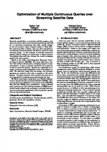
Single Query

Comparison of overall communication cost (does not include growth message communication costs) incurred by the adaptive algorithm against the uniform static allocation measuring cost for 21hrs. The CQ monitors the average traffic level with varying precision constraint δ

Impact of Message Latency  Vary the maximum latency tolerance and measure the

fraction of updates arriving within the tolerance  Updates exceeding the latency allowance occur only about once every 65.7 minutes, 99:997% reached

Conclusions  Experimental results show that the proposed



  

approach saves communication cost at fine granularity by individually adjusting precision constraints The experiments were based on simple examples of network traffic with a few hosts. The values of S and T were determined experimentally. Effect of variation of T on the on quality of answers is not available. Evaluating S experimentally, may not be feasible in all cases The streamed update period Pi = T / Ni takes into consideration only the updates in the last T time units. Considering the complete history of updates (Kalman filter) might show interesting results !

Thanks!