Distributed Evaluation of Continuous Equi-join Queries ... - Stratos Idreos

Distributed Evaluation of Continuous Equi-join Queries over Large Structured Overlay Networks

by Stratos Idreos A thesis submitted in fulfillment of the requirements for the Master of Computer Engineering

Department of Electronic and Computer Engineering Technical University of Crete, GR73100 Chania, Greece September 17, 2005

Contents 1 Introduction 1.1 Contributions . . . . . . . . . . . . . . . . . . . . . . . . . . . . . 1.2 Organization of the thesis . . . . . . . . . . . . . . . . . . . . . . 2 Structured Overlay Networks 2.1 Distributed Hash Tables . . . 2.2 The Chord DHT protocol . . 2.3 Extensions to the Chord API 2.4 Summary . . . . . . . . . . .

. . . .

. . . .

. . . .

. . . .

. . . .

. . . .

. . . .

. . . .

. . . .

. . . .

. . . .

. . . .

. . . .

. . . .

. . . .

. . . .

. . . .

. . . .

. . . .

. . . .

6 7 7 9 9 10 12 13

3 System model and data model 14 3.1 Network Architecture . . . . . . . . . . . . . . . . . . . . . . . . 14 3.2 Data model and Query Language . . . . . . . . . . . . . . . . . . 14 3.3 Summary . . . . . . . . . . . . . . . . . . . . . . . . . . . . . . . 16 4 Algorithms 4.1 Two-level indexing . . . . . . . . . . . . . . . . . . . . 4.2 Tuple indexing . . . . . . . . . . . . . . . . . . . . . . 4.3 The single-attribute index algorithm . . . . . . . . . . 4.3.1 Indexing a query at the attribute level . . . . . 4.3.2 Handling tuple insertions at the attribute level 4.3.3 Processing rewritten queries at the value level . 4.3.4 Handling tuple insertions at the value level . . 4.3.5 Local query indexing and grouping . . . . . . . 4.3.6 Choosing the index attribute . . . . . . . . . . 4.4 The double-attribute index algorithms . . . . . . . . . 4.4.1 Common steps in all DAI algorithms . . . . . . 4.4.2 The DAI-Q algorithm . . . . . . . . . . . . . . 4.4.3 The DAI-T algorithm . . . . . . . . . . . . . . 4.5 The DAI-V algorithm . . . . . . . . . . . . . . . . . . 4.6 Delivering notifications . . . . . . . . . . . . . . . . . . 4.7 Optimizations . . . . . . . . . . . . . . . . . . . . . . . 4.7.1 The join fingers routing table . . . . . . . . . . 4.7.2 Balancing the load at the attribute level . . . .

1

. . . . . . . . . . . . . . . . . .

. . . . . . . . . . . . . . . . . .

. . . . . . . . . . . . . . . . . .

. . . . . . . . . . . . . . . . . .

. . . . . . . . . . . . . . . . . .

. . . . . . . . . . . . . . . . . .

17 17 19 20 20 21 22 22 24 25 26 26 28 28 28 31 33 33 33

4.8

Summary . . . . . . . . . . . . . . . . . . . . . . . . . . . . . . .

35

5 Experiments 5.1 General set-up of the experiments . . . . . . . 5.2 Evaluation of the API . . . . . . . . . . . . . 5.3 Network traffic and JFRT effect . . . . . . . . 5.4 Varying the number of indexed queries . . . . 5.5 Evaluating the index attribute choice in SAI . 5.6 Effect of the bos ratio . . . . . . . . . . . . . 5.7 Evaluation of the replication scheme . . . . . 5.8 Total load created . . . . . . . . . . . . . . . 5.9 Load distribution . . . . . . . . . . . . . . . . 5.10 Parameters that affect load distribution . . . 5.11 Summary . . . . . . . . . . . . . . . . . . . .

. . . . . . . . . . .

. . . . . . . . . . .

. . . . . . . . . . .

. . . . . . . . . . .

. . . . . . . . . . .

. . . . . . . . . . .

. . . . . . . . . . .

. . . . . . . . . . .

. . . . . . . . . . .

. . . . . . . . . . .

. . . . . . . . . . .

36 36 37 38 40 41 42 43 45 47 50 54

6 Related work 6.1 Distributed and Parallel Databases . . . . . 6.2 P2P Databases . . . . . . . . . . . . . . . . 6.3 Continuous Queries and Stream Processing 6.4 Pub/Sub Networks . . . . . . . . . . . . . . 6.5 Summary . . . . . . . . . . . . . . . . . . .

. . . . .

. . . . .

. . . . .

. . . . .

. . . . .

. . . . .

. . . . .

. . . . .

. . . . .

. . . . .

. . . . .

55 55 56 57 58 60

7 Conclusions and future work

. . . . .

61

2

List of Figures 2.1

An example of a network

. . . . . . . . . . . . . . . . . . . . . .

10

3.1

An example of a network

. . . . . . . . . . . . . . . . . . . . . .

15

4.1 4.2 4.3 4.4 4.5

Inserting a tuple of a binary An example with SAI . . . Duplicate notifications . . . An example with DAI-T . . Moving an identifier . . . .

. . . . .

19 23 27 29 34

5.1 5.2 5.3 5.4

Recursive vs. iterative design for the multiSend function . . . . . Traffic cost and JF RT effect . . . . . . . . . . . . . . . . . . . . Effect of the number of indexed queries in network traffic . . . . Comparison of the various index attribute selection strategies in SAI . . . . . . . . . . . . . . . . . . . . . . . . . . . . . . . . . . Effect of varying the bos ratio . . . . . . . . . . . . . . . . . . . . Effect of the replication scheme in filtering load distribution . . . Effect of the replication scheme in storage load distribution . . . Effect of window size and installed queries in total evaluator filtering load . . . . . . . . . . . . . . . . . . . . . . . . . . . . . . . Effect of window size and installed queries in total evaluator storage load . . . . . . . . . . . . . . . . . . . . . . . . . . . . . . . . T F and T S load distribution comparison for all algorithms . . . Total filtering and total storage load distribution comparison for the two level indexing algorithms . . . . . . . . . . . . . . . . . . Effect in filtering load distribution of increasing the frequency of incoming tuples . . . . . . . . . . . . . . . . . . . . . . . . . . . . Effect in filtering load distribution of increasing the number of indexed queries . . . . . . . . . . . . . . . . . . . . . . . . . . . . Effect in filtering load distribution of increasing the network size Effect in filtering load distribution of increasing the network size for the most loaded nodes . . . . . . . . . . . . . . . . . . . . . . Effect in filtering load distribution of DAI-V of increasing the network size, queries or tuples . . . . . . . . . . . . . . . . . . . .

37 38 40

5.5 5.6 5.7 5.8 5.9 5.10 5.11 5.12 5.13 5.14 5.15 5.16

relation . . . . . . . . . . . . . . . . . . . .

3

. . . . .

. . . . .

. . . . .

. . . . .

. . . . .

. . . . .

. . . . .

. . . . .

. . . . .

. . . . .

. . . . .

. . . . .

. . . . .

. . . . .

. . . . .

41 43 44 45 46 47 48 50 51 52 52 53 54

List of Tables 4.1

A comparison of all algorithms . . . . . . . . . . . . . . . . . . .

4

32

Abstract We study the problem of continuous relational query processing in Internetscale overlay networks realized by distributed hash tables. We concentrate on the case of continuous two-way equi-join queries. Joins are hard to evaluate in a distributed continuous query environment because data from more than one relations is needed, and this data is inserted in the network asynchronously. Each time a new tuple is inserted, the network nodes have to cooperate to check if this tuple can contribute to the satisfaction of a query when combined with previously inserted tuples. We propose a series of algorithms that initially index queries at network nodes using hashing. Then, they exploit the values of join attributes in incoming tuples to rewrite the given queries into simpler ones, and reindex them in the network where they might be satisfied by existing or future tuples. We present a detailed experimental evaluation in a simulated environment and we show that our algorithms are scalable, balance the storage and query processing load and keep the network traffic low.

Chapter 1

Introduction We are interested in the problem of relational query processing in wide-area networks such as the Internet and the Web. This is an important research area with applications to e-learning [50], P2P databases [34], monitoring [32] and stream processing [47]. We envision large P2P overlay networks where information is inserted and stored in the form of relational tuples and is queried with SQL queries. Each node keeps a fraction of the total data tuples. Tuples of a given relation can be distributed among various nodes. In this thesis we concentrate on continuous relational query processing and present algorithms for continuous two-way equi-join queries. Join queries have traditionally been the study of many query optimization efforts. Distributed evaluation of join queries is very challenging, mainly due to the fact that data from different parts of the network have to be combined to answer a query. We consider this thesis to be our first step in contributing to the vision of relational P2P databases: a set of unified protocols that will fully support SQL over P2P networks. Current work on continuous relational queries has mostly emphasized system design and query evaluation for the centralized case [66, 44, 17, 47, 57]. Recent papers [27, 32] and the present thesis study continuous relational query processing in its natural habitat dictated by target applications: distributed, Internet-scale environments realized by technologies building on distributed hash tables (DHTs) [60]. The only system so far that implements join algorithms on top of DHTs is PIER [34] but this is done only for the case of one-time queries. The case of continuous join queries is a different one and cannot be captured by the algorithms presented in [34]. PeerCQ is another interesting system proposed for continuous queries over DHTs [27]. PeerCQ does not consider the relational data model and the SQL query language, and assumes that data is not stored in a DHT but is kept locally in external data sources. In PeerCQ, the DHT infrastructure is nicely utilized to achieve a good distribution of the responsibilities for monitoring external data sources and evaluating queries. To the best of our knowledge, this thesis is the first one that presents algorithms for continuous relational join queries on top of DHTs where DHT nodes are fully utilized to store data tuples and run collaborative query processing protocols. 6

1.1

Contributions

The contributions of this thesis are the following. We present four distributed algorithms for evaluating continuous two-way equi-join queries over DHTs. In our algorithms, when a node poses a continuous query, the query is indexed somewhere in the network and waits for incoming tuples. As new tuples are inserted, the network nodes cooperate to deliver a notification to the node that posed the query. All algorithms in the thesis use a two-level indexing mechanism to index queries and tuples. In the first level, nodes use attribute names prefixed by relation names to index a query or a tuple. In the second level, nodes utilize attribute values in order to achieve a better load distribution. The two-level indexing mechanism is exploited by a two-phase query evaluation algorithm. The emphasis of our algorithms is twofold. We try to distribute the load of evaluating continuous join queries to as many nodes as possible and, at the same time, keep the cost in terms of overlay hops low. We show the tradeoff between achieving load distribution and performing query evaluation with as little network traffic as possible. Each algorithm we studied offers a particular way to resolve this tradeoff, and it might be appropriate for applications with relevant characteristics. One of our technical contributions is the introduction of appropriate metrics for capturing individual node load and total system load in our environment. The challenges presented by continuous query processing should not be underestimated. When the number of installed queries increases, the total query processing load and network traffic created by incoming tuples increases as well. Similarly, when the rate of incoming tuples in a given time window increases, a higher amount of installed queries will be triggered, leading to a higher query processing load and network traffic. Our simulations show that our algorithms are scalable to such changes. Even when these changes take place simultaneously, our algorithms manage to distribute the query answering load gracefully among existing nodes. Another aspect of scalability is also clearly demonstrated in our work. When the overlay network grows, query processing becomes easier since new nodes relieve other nodes by taking a portion of the existing workload. The experiments we present use Chord [60] as the underlying DHT, due to its relative simplicity, and appropriateness for equi-join queries. However, our ideas are DHT-agnostic: they will work with any DHT extended with the APIs we define. Recent distributed data structure proposals such as [20, 54, 37] that can handle equality queries and range queries efficiently can also be extended to handle two-way join queries (with equality or other comparison operators) in a straightforward way using our approach.

1.2

Organization of the thesis

The organization of the thesis is as follows. In Chapter 2 we generally discuss about DHTs and we briefly describe Chord and our proposed extensions to the Chord API. Chapter 3 gives our assumptions regarding system and data model.

7

Chapter 4 discusses alternative indexing and query evaluation algorithms. It also explains how notifications are stored and delivered and discusses optimizations while in Chapter 5 we present a detailed experimental evaluation. Chapter 6 discusses related work and finally, Chapter 7 concludes the thesis.

8

Chapter 2

Structured Overlay Networks In this chapter we give a general description of the new generation of structured overlay networks, called distributed hash tables (DHTs). We describe in detail the Chord overlay network that we use to build our algorithms and then we present a simple API that we have designed and implemented on top of Chord to achieve more efficient routing of messages.

2.1

Distributed Hash Tables

The success of P2P protocols and applications such as Napster and Gnutella motivated researchers from the distributed systems, networking and database communities to look more closely into the core mechanisms of these systems and investigate how these could be supported in a principled way. This quest gave rise to a new wave of distributed protocols, collectively called distributed hash tables [60, 53, 55, 2, 33, 48, 7]. DHTs are structured P2P systems. DHTs attempt to solve the following look-up problem: Let X be some data item stored at some distributed dynamic network of nodes. Find data item X. The core idea in all DHTs is to solve this look-up problem by offering some of form of distributed hash table functionality: assuming that data items can be identified using unique numeric keys, DHT nodes cooperate to store keys for each other (data items can be actual data or pointers). Implementations of DHTs offer a very simple interface consisting of two operations: • put(ID, item). This operation inserts item with key ID and value item in the DHT. • get(ID). This operation returns a pointer to the DHT node responsible for key ID. 9

Figure 2.1: An example of a network Although the DHTs available in the literature differ in their technical details, all of them address the following central questions: • How do we map keys to nodes? Keys and nodes are identified by a binary number. Keys are stored at one or more nodes with identifiers “close” to the key identifier in the identifier space. • How do we route queries for keys? Any node that receives a query for key k, returns the data item X associated with k if it owns k, otherwise it forwards k to a node with identifier “closer” to k using only local information. • How do we deal with dynamicity? DHTs are able to adapt to node joins, leaves and failures and update routing tables with little effort. In the rest of this section we give a short description of Chord and of the API that we created on top of Chord.

2.2

The Chord DHT protocol

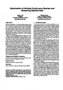
Each node n in the network owns a unique key, denoted by Key(n). For example, this key can be created by the public key of the node and/or its IP address. Each item i also has a key, denoted by Key(i). For example, in a file-sharing application, where the items are files, the name of a file can be the key (this is an application-specific decision). In our case the items are queries and tuples and keys are determined in ways to be explained later. Chord uses a variation of consistent hashing [38] to map keys to nodes. In the consistent hashing scheme each node and data item is assigned a m-bit identifier where m should be large enough to avoid the possibility of different items hashing to the same identifier (a cryptographic hashing function such as SHA-1 can be used). Each node n is assigned an identifier, denoted by id(n), that is computed by hashing its key Key(n). Similarly, each item i is assigned an identifier, denoted by id(i), by hashing Key(i). Identifiers are ordered in an identifier circle (ring) module 2m i.e., from 0 to 2m − 1. Figure 2.1 shows an example of an identifier circle with 64 identifiers (m = 6) but only 10 nodes. Keys are mapped to nodes in the identifier circle as follows. Let Hash be the consistent hash function used. Key k is assigned to the the first node which 10

is equal or follows Hash(k) in the identifier space. For example in the network shown in Figure 2.1, a key with identifier 8 would be stored at node N 8. In other words, key k is assigned to the node whose identifier is the first identifier clockwise in the identifier circle starting from Hash(k). This node is called the successor node of identifier Hash(k) and is denoted by successor(Hash(k)). We will often say that this node is responsible for key k. In our example, node N 32 would be responsible for all keys with identifiers in the interval (21, 32]. If each node knows its successor, a query for locating the node responsible for a key k can always be answered in O(N ) steps where N is the number of nodes in the network. To improve this bound, Chord maintains at each node a routing table, called the finger table, with at most m entries. Each entry j in the finger table of node n, points to the first node s on the identifier circle that succeeds identifier Hash(Key(n)) + 2j−1 . These nodes (i.e., successor(Hash(Key(n)) + 2j−1 ) for 1 ≤ j ≤ m) are called the fingers of node n. Since fingers point at repeatedly doubling distances away from n, they can speed-up search for locating the node responsible for a key k. If the finger tables have size O(log N ), then finding a successor of a node n can be done in O(log N ) steps with high probability [60]. To simplify joins and leaves, each node n maintains a pointer to its predecessor node i.e., the first node counter-clockwise in the identifier circle starting from n. When a node n wants to join a Chord network, it finds a node n0 that is already in the network using some out-of-band means, and then asks n0 to help n find its position in the network by discovering n’s successor [61]. Every node runs a stabilization algorithm periodically to learn about nodes that have recently joined the network. When n runs the stabilization algorithm, it asks its successor for the successor’s predecessor p. If p has recently joined the network then it might end-up becoming n’s successor. Each node n periodically runs two additional algorithms to check that its finger table and predecessor pointer is correct [61]. Stabilization operations may affect queries by rendering them slower (because successor pointers are correct but finger table entries are inaccurate) or even incorrect (when successor pointers are inaccurate). However, assuming that successor pointers are correct and the time it takes to correct finger tables is less than the time it takes for the network to double in size, one can prove that queries can still be answered correctly in O(log N ) steps with high probability [61]. To deal with node failures and increase robustness, each Chord node n maintains a successor list of size r which contains n’s first r successors. This list is used when the successor of n has failed. In practice even small values of r are enough to achieve robustness [61]. If a node chooses to leave a Chord network voluntarily then it can inform its successor and predecessor so they can modify their pointers and, additionally, it can transfer its keys to its successor. It can be shown that with high probability, any node joining or leaving a Chord network can use O(log2 N ) messages to make all successor pointers, predecessor pointers and finger tables correct [60].

11

2.3

Extensions to the Chord API

In this section we present the API we use to build our algorithms. It is a simple extension of the standard API of the Chord protocol to support routing features that are repeatedly used by our algorithms. To facilitate message sending between two nodes we will use the function send(msg, I) to send message msg from some node to node Successor(I), where I is a node identifier. Function send() is similar to Chord function lookup(I) [60] with msg piggy backed, and costs O(logN ) overlay hops for a network of N nodes. When function send(msg, I) is invoked by node n, it works as follows. Node n contacts node n0 , where id(n0 ) is the greatest identifier contained in the finger table of n, for which id(n0 ) ≤ I holds. Upon reception of a send() message by a node x, I is compared with id(x). If id(x) < I, then node x just forwards the message by calling send(msg, I) itself. If id(x) ≥ I, then x processes msg since it is the intended recipient. Our algorithms also require that a node is capable of sending the same message to a group of nodes. This group is created dynamically (i.e., each time a tuple insertion or a query submission takes place), so multicast techniques for DHTs such as [8] are not applicable. The obvious way to handle this over Chord is to create k different send() messages, where k is the number of different nodes to be contacted, and then locate the recipients of the message in an iterative fashion using O(k log N ) messages. We have implemented this algorithm for comparison purposes. We have also designed and implemented function multiSend(msg, L), where L is a list of k identifiers, that can be used to send message msg to the k elements of L in a recursive way. It is used to send msg to nodes n1 , n2 , ..., nk such as that nj = Successor(Ij ), where 1 ≤ j ≤ k. When function multiSend() is invoked by node n, it works as follows. Initially n sorts the identifiers in L in ascending order clockwise starting from id(n). Subsequently n contacts n0 , where id(n0 ) is the greatest identifier contained in the finger table of n, for which id(n0 ) ≤ head(L) holds, where head(L) is the first element of L. Upon reception of a multiSend() message, by a node x, head(L) is compared with id(x). If id(x) < head(L), then node x just forwards msg by calling multiSend() again. If id(x) ≥ head(L), then node x processes msg since this means that it is one of the intended recipients contained in list L (in other words, x is responsible for key head(L)). Then x creates a new list L0 from L in the following way. x deletes all elements of L that are smaller or equal to id(x), starting from head(L), since node x is responsible for them. In the new list L0 that results from these deletions, we have that id(x) < head(L0 ). Finally, node x forwards msg to node with identifier head(L0 ) by calling multiSend(msg, L0 ). This procedure continues until all identifiers are deleted form L. The cost for contacting all k nodes is again O(k log N ) but the recursive approach has in practice a significantly better performance than the iterative method as we show in Section 5. Function multiSend() can also be used as, multiSend(M, L), where M is a set of k messages and L is a set of k identifiers. For each Lj , the function will deliver message Mj to Successor(Lj ) as in the previous paragraph. 12

2.4

Summary

In this chapter we outlined the key ideas of current structured overlay networks. More precisely we presented the Chord DHT protocol which is the DHT protocol used to present our algorithms. We also introduced an API to enhance the routing capabilities of DHTs with respect to specific requirements of our algorithms. In the next chapter we present the assumption regarding the architecture of the network and the supported data model.

13

Chapter 3

System model and data model In this chapter we describe in detail the architecture of the network we assume. We provide details regarding the role of the various nodes that participate in the overlay and we also discuss the data model and query types supported by the algorithms we propose in this thesis.

3.1

Network Architecture

We assume an overlay network where all nodes are equal, as they run the same software and they have the same rights and responsibilities. Nodes are organized according to the Chord DHT protocol and are assumed to have synchronized clocks. In practice, nodes will run a protocol such as NTP [10] and achieve accuracies within few milliseconds. Each node can insert data and pose continuous queries. Each time new data is inserted the network nodes cooperate to create notifications and notify nodes that have inserted relevant queries. A high level view of the network architecture is shown in Figure 3.1.

3.2

Data model and Query Language

In this thesis data is described using the relational data model and is inserted in the system in the form of data tuples. As in PIER [34], different schemas can co-exist but schema mappings are not supported. Continuous queries are formed using the SQL query language. We consider the case of two-way equi-joins i.e., SQL queries of the form: Select R.A1 , . . . , R.Aκ , S.B1 , . . . , S.Bλ From R, S Where α = β

14

Figure 3.1: An example of a network where R and S are relations with schemas R(A1 , . . . , Aν ) and S(B1 , . . . , Bµ ), 1 ≤ κ ≤ ν, 1 ≤ λ ≤ µ and α is an expression (e.g., arithmetic, string) involving only attributes of R and possibly constants, and β is an expression involving only attributes of S and possibly constants. We distinguish two types of queries depending on the form of α and β. If α and β involve a single attribute of R and S (e.g., Ai and Bj respectively) and equality α = β has a unique solution over dom(Ai ) × dom(Bj ) then we say q is of type T1 . If any of α or β involve more than one attributes of R and S then we say q is of type T2 . We show how to evaluate such queries without first transforming them to simple equi-joins using generalized projection. Each tuple t has a time parameter called publication time, denoted by pubT (t), representing the time that the tuple was inserted into the system. In addition, each query q has a time parameter, called insertion time, denoted by insT (q) that shows the creation time of q. A tuple t can trigger a query q iff pubT (t) ≥ insT (q) i.e., only tuples inserted after a query was posed can trigger it. Whenever the Where clause of a query is satisfied, an answer is computed and this is the notification sent to the query subscriber. Each query q has a unique key, denoted by Key(q), that is created from the key of the node n that poses it, by concatenating a positive integer to Key(n). Like [34], we assume a “best-effort” semantics for query evaluation and leave all the handling of failures, partitions etc. to the underlying DHT. Example. Consider an e-learning network such as EDUTELLA where nodes join the network for the purposes of sharing learning material [19]. Let us assume the learning material consists of research papers that are inserted in the overlay once they are published. Each paper can be described by a set of tuples using the following simple schema: Document(Id, T itle, Conf erence, AuthorId), Authors(Id, N ame, Surname) The following query asks that its subscriber be notified whenever author Smith publishes a new paper: Select D.T itle, D.Conf erence 15

From Document as D, Authors as A Where D.AuthorId = A.Id and A.Surname = Smith

3.3

Summary

In this chapter we described the assumed architecture of our overlay network. We presented the data model and the query types that our current algorithms support. We also described the time semantics, i.e., when a new tuple can trigger an already indexed query. In the next chapter we continue with a detailed description of our algorithms.

16

Chapter 4

Algorithms In this chapter we present a detailed description of our algorithms for evaluating two-way equi-join queries. First we motivate our general design goals by presenting a few naive solutions that tend to collect the query processing load to a small part of the network. Then we continue with the description of the four algorithms and examples. Finally, we also introduce a set of optimizations that can be applied to all algorithms to improve the generated network traffic and load distribution.

4.1

Two-level indexing

One of the main challenges when designing a distributed query processing algorithm is to generate as little load as possible in the network and to distribute this load fairly among existing nodes. Assume a continuous two-way join query with the join condition R.B = S.E. The goal is to index the query in such a way, so that when new tuples are inserted, the query and the tuples will meet to create notifications. Indexing a query amounts to storing the query at one or more nodes of the overlay. We could index queries to a globally known node or set of nodes, but this would eventually overload these nodes. In a P2P environment we want as many nodes as possible to contribute some of their resources (storage, cpu, bandwidth, etc.) for achieving the overall network functionality. The resource contribution of each node will obviously depend on its capabilities, its gains from participating in the network etc. In this thesis we make the simplifying assumption that all nodes are equivalent and can contribute to query evaluation in identical ways. We choose to index a query using identifiers that are related to the query. This is a useful property since a tuple that should trigger a query q, is also related to the query q, for example, they both refer to the same relation. In this way, it is easy to make an incoming tuple meet the appropriate queries without any global knowledge or broadcasting. The difficulty with join queries is that a join condition, like the one in our ex-

17

ample, gives us little flexibility. For example, let us consider the simpler case of continuous select-project queries with a Where clause of the form R.B = value. In this case, we can simply assign the query to the successor node x of the identifier Hash(R + B + value). We use the operator + to denote the concatenation of string values. Relevant tuples will arrive at x in the same way, and we have to worry only for skewed values regarding load distribution. With this solution to select-project queries in mind, how do we index a query with a join condition like R.B = S.E? One way could be to index the query to the successor nodes x1 and x2 of the identifiers Hash(R) and Hash(S) respectively. Incoming tuples could then be indexed according to their relation name, and some kind of communication is required between x1 and x2 to create notifications. The problem with such a solution is that the query processing load is gathered to a small subset of the set of network nodes, i.e., to as many nodes as the number of distinct relations in the schema. This means that as the network size grows, the network utilization (i.e., the percentage of nodes participating in query processing) drops. The next logical step is to also use the attribute names in the indexing scheme i.e., x1 , x2 can be the successor nodes of the identifiers Hash(R + B) and Hash(S + E) respectively. Now we can expect a better distribution of the query processing load but again the total number of nodes contributing to query processing is limited (bounded by the total number of attributes in the schema). Another approach would be to index a join query according to an expression combining the two join attributes, i.e., to the successor node of Hash(R.B+S.E) for our example. However, new tuples would have to reach all pair combinations of the attributes of different relations of the schema, to guarantee completeness. Although evaluating locally a query is now very easy since we have the two relations in one node, the main disadvantage of this method is again the fact that the number of nodes that are responsible for query processing is bounded; this time by the possible join pairs. All the previous solutions have the disadvantage that only a subset of the set of network nodes sustain the total query processing load. As with select-project queries we would like to use the various values that the join attributes can take in order to distribute this load. However, these values are not known at the time that the query is inserted but are revealed to us as tuples arrive. The algorithms we propose exploit this fact by using the values in incoming tuples that trigger a query in order to distribute the query processing load. The four algorithms we will present are based on a two-level indexing mechanism to index queries and tuples. In the first level (attribute level ) nodes use the names of attributes prefixed by their relation names to index a query or a tuple. In the case of a query, those attributes are among the ones involved in the join condition. In the second level of indexing (value level ), nodes utilize attribute values in order to achieve a better load distribution. A high level description of the indexing and query processing algorithms we present is as follows. To pose a query q, a node indexes q at the attribute level where q is stored waiting for tuples to trigger it. When a node wants to insert a tuple, it indexes the tuple both at the attribute and at the value level. As tuples of 18

Figure 4.1: Inserting a tuple of a binary relation the involved relations are inserted at the attribute level, the indexed queries are triggered, rewritten and reindexed at the value level according to the values of their join attributes in the incoming tuples. More precisely, one of the two join attributes is replaced in the join condition by its value in the incoming tuple. In this way, the join query is reduced to a simple select-project query that enters in the network (reindexing) and waits to be triggered. Thus, a single join query q is evaluated by multiple nodes that share the query processing load at the value level by evaluating the multiple select-project queries that have been created from different values of the join attributes. Our algorithms result in the allocation of two roles to network nodes: the role of query rewriters and the role of query evaluators. A node can play both, one or none of these roles depending on the queries and tuples that are present in the network, and the node’s position in the identifier space. The four algorithms we propose can be classified into two categories according to how query indexing takes place. We present one algorithm that uses one of the two join attributes to index a query (single-attribute indexing) and three algorithms that use both join attributes (double-attribute indexing) so as to exploit the possibility to achieve a better query processing load distribution. We continue our presentation by explaining how tuples are indexed in our proposal. Sections 4.3, 4.4 and 4.5 discuss how join queries are indexed and how nodes react upon receiving a new tuple in order to trigger the appropriate queries.

4.2

Tuple indexing

Our tuple indexing protocol is a variation of hash partitioning. Assume a relation R over h attributes and a node x1 that wants to insert a new tuple t. Let {A1 , A2 , ...., Ah } be the attributes in t with values {v1 , v2 , ...., vh } respectively. For each Ai , x1 computes the following two identifiers: AIndexi = Hash(R + Ai ) V Indexi = Hash(R + Ai + vi ) 19

When the value of an attribute is numeric (e.g., an integer), this value is also treated as a string. For each Ai , tuple t will be indexed twice: once according to AIndexi at the attribute level, and once according to V Indexi at the value level. Thus a set I of 2h identifiers is created by node x1 . For each AIndexi , x1 creates a message al-index(t, Ai ). Similarly for each V Indexi , x1 creates a message vl-index(t, Ai ). Attribute Ai is included in the messages so that node x2 that receives t can tell which attribute was used to index t to x2 (used for local processing); this attribute will be denoted by IndexA(t). Thus, a set M of 2h messages is created and x1 calls function multiSend(M, I) to index t in 2h ∗ O(logN ) overlay hops. A complete example of inserting a tuple is shown in Figure 4.1. The way a node reacts, upon receiving a tuple, depends on the algorithm and on the indexing level that the tuple was received. These details will be discussed in Sections 4.3, 4.4 and 4.5 where we describe query indexing algorithms and how they are used to evaluate continuous two-way equi-join queries. In general, a tuple is never stored at the attribute level, it just triggers the queries indexed at a node. At the value level, a node may store a tuple or not, and may try to trigger locally stored queries or not depending on the algorithm.

4.3

The single-attribute index algorithm

Let us now describe our first algorithm, the single-attribute index algorithm (SAI). To pose a query q of type T1 , a node n indexes q by one of the two join attributes at the attribute level. Node x that receives q, stores it locally and when tuples that trigger q arrive at x, x rewrites and reindexes q to nodes that are capable to create notifications at the value level.

4.3.1

Indexing a query at the attribute level

Indexing a query q at the attribute level proceeds as follows. First, node n chooses one of the join attributes of q which will be used to index q. For the moment, we assume that this choice is random; more detailed criteria are discussed in Section 4.3.6. We call this attribute the index attribute of q and the relation that it belongs to the index relation of q, and denote them by IndexA(q) and IndexR(q) respectively. The remaining join attribute is called the load distributing attribute of q and its relation the load distributing relation of q, denoted by DisA(q) and DisR(q) respectively. As we will see below, the values of attribute DisA(q) of relation DisR(q) will be used to distribute the query processing load generated during the evaluation of q, hence our terminology. Then, node n creates the identifier AIndex that determines the node that the query will be indexed to. This is done as follows: AIndex = Hash(IndexR(q) + IndexA(q)) Notice that this identifier is calculated exactly in the same way as an AIndex identifier of a tuple which means that future tuples of relation IndexR(q) will meet the query q at the attribute level. 20

Then, node n creates the message msg = query(q, Id(n), IP (n)). Arguments Id(n) and IP (n) are used when delivering notifications back to n (see Section 4.6). Finally, node n calls the function send(msg,AIndex) to index q at the attribute level with complexity O(logN ). Node Successor(AIndex) that receives msg is called the rewriter of q. The rewriter node of q stores q in the local attribute-level query table (ALQT ) and waits for tuples to trigger it. The role of a rewriter node is not to compute the join itself, but to distribute the load of computing joins, creating notifications and delivering them. Each query has one rewriter and all queries with the same index attribute have the same rewriter.

4.3.2

Handling tuple insertions at the attribute level

In SAI, an incoming tuple is indexed both at the attribute and at the value level according to the protocol of Section 4.2. We will first describe what happens at the attribute level. Assume a node x that receives a tuple t at the attribute level with the message al-index(t, IndexA(t)). Node x searches its ALQT for queries that are triggered by t. The result is a set of k join queries. Since these queries were in the local ALQT , node x is their rewriter node. For each query qi , node x owns information on one of the two relations needed to compute the join, namely on IndexR(qi ). This information is the new tuple t. Another node has to be contacted then, where tuples of relation DisR(qi ) are stored or are expected to arrive. Since qi is an equi-join query, the only suitable tuples are the ones where the value of DisA(qi ) satisfies the join condition of qi after IndexA(qi ) has been replaced with its value in t. If valDA(qi , t) is that value, then this node is the successor node of the following identifier: V Index(qi ) = Hash(DisR(qi ) + DisA(qi ) + valDA(qi , t)) Notice that the way this identifier is calculated is similar to how a V Index identifier of a tuple is calculated which means that tuples that are indexed at the value level will meet the query. So this node has the rest of the tuples needed to evaluate the join due to how tuples are indexed at the value level. We call this node the evaluator of the query for the value valDA(qi , t). A query q has as many evaluators, as the distinct values of attribute IndexA(q). Let us now discuss what a rewriter sends to an evaluator. Each query qi is rewritten according to the incoming tuple t. The resulting query qi0 will produce the same notifications, when sent to an evaluator, as if t and qi had both arrived there. To create qi0 , each attribute of IndexR(qi ) in the Select and Where clause of qi , is replaced by its corresponding value in t. Assume the query Select R.A, S.B F rom R, S W here R.C = S.C which is triggered at the attribute level by a tuple S(3, 4, 7). The rewritten query will be Select R.A, 4 F rom R W here R.C = 7. Thus, the original query is reduced to a simple select-project query which will be send (reindexed) at the Successor(Hash(R + C +0 70 )). In this way, the rewriter node x rewrites all k triggered queries and for each rewritten query qi0 it creates a message join(qi0 ). Thus, a set M of k 21

messages and a set I of k V Index identifiers are created. Then, node x calls the multiSend(M,I) function to reindex the rewritten queries at the value level which costs k ∗ O(logN ) overlay hops.

4.3.3

Processing rewritten queries at the value level

We will now discuss how a node x at the value level reacts upon receiving a rewritten query q 0 with a join(q 0 ) message. Assume that q 0 was created by query q when tuple t of relation IndexR(q) arrived at the attribute level. First, x has to check whether it locally stores any matching tuples of DisR(q) so as to create notifications, i.e., tuples that were inserted in the network after q. In addition, node x has to remember the fact that q 0 arrived in order to be able to create notifications in the future, when more tuples of DisR(q) arrive. Thus, x stores q 0 in its value-level query table (V LQT ). This last step is necessary only if this is the first time that x receives q 0 whereas if there is already a same query q 0 stored at x, then x need only to store the information related to tuple t. Whether a rewritten query is already stored or not can be easily determined using the unique keys of the queries. As we have already discussed each query q has a unique key, denoted by key(q). A rewritten query q 0 of q has a different key than key(q). This new key is calculated at the time that q is triggered at the attribute level by t to create q 0 as follows. If A1, A2, ..., Al are the attributes of IndexR(q) in the Select clause of q, then the key of the rewritten query is Key(q 0 ) = Key(q) + v1 + v2 + ... + vl + valDA(q, t), where vj is the value of Aj in the tuple t that triggered q for j = 1, 2, ..., l. In this way, , an evaluator x will store a new rewritten query if no rewritten query with the same key has ever arrived to n. If there is a query q 0 with the same key, then only pubT (t) is stored along with q 0 . The time information is necessary when creating notifications. The way keys are created for rewritten queries guarantees that two rewritten queries will have the same key if they are created from the same query q but by different tuples that have the same value for IndexA(q).

4.3.4

Handling tuple insertions at the value level

Let us now see what happens as tuples arrive at the value level where they meet rewritten queries that have been reindexed. Assume a node x that receives a tuple at the value level with a message vl-index(t, IndexA(t)). First, node x checks if there is any rewritten query q 0 in its V LQT that is triggered by the new tuple. For each triggered query a notification is created. In addition, tuple t is also stored in the local value-level tuple table (V LT T ). Storing tuples at the value level is necessary for the completeness of SAI. As an example assume the following series of events: (a) a query q is indexed, (b) a tuple t of DisR(q) is inserted and stored at node x (at the value level), and (c) a tuple of IndexR(q) is inserted causing query q to be rewritten and reindexed to x. If t is not stored at x then a notification will be lost.

22

Figure 4.2: An example with SAI

23

A complete example with SAI is shown in Figure 4.2. Events take place from left to right, i.e., initially query q is indexed and then tuples arrive. For readability, only the steps that affect query q are shown. Notice that while in Step 3 a notification is created by a tuple that meets a rewritten query at the value level, in Step 5 the opposite happens.

4.3.5

Local query indexing and grouping

Since a large number of queries are expected to be similar, i.e., reference the same relations, all queries that have equivalent join condition are grouped together at each rewriter and evaluator node. Equivalence is easy to determine during parsing for queries of type T1 . Grouping queries is useful for minimizing the local computation cost and the network cost. Similar queries are triggered in a single step. In addition, reindexing can also be done with only one message for multiple queries since for the same incoming tuple all similar queries will require the same evaluator. Locally tuples and queries are stored in hash table based data structures. Let us shortly describe this data structures that are designed so as to efficiently handle incoming requests. The ALQT that is used by rewriter nodes to store queries at the attribute level, is a two level hash table. At the first level, queries are indexed according to their index attribute while at the second level the string values of join conditions are used as keys. In this way, each time a new tuple arrives at a rewriter node, the index attribute of the tuple is used to find all triggered queries in one step using the first level of the local ALQT . At the second level queries are grouped according to their join condition so it is then easy for the rewriter node to handle (rewrite/reindex) all the triggered queries by avoiding redundant operations for multiple queries in the same group. At the value level evaluators nodes maintain the V LQT which is a two level hash table used to store the rewritten queries that these nodes receive. At the first level rewritten queries are indexed according to their load distributing attribute, while at the second level according to the value that this attribute must take so as to satisfy their join condition. In this way, when a new tuple arrives at an evaluator node, the rewritten queries that are possible to match the new tuple can be found in one step at the first level of the local V LQT using the index attribute of the new tuple. Then with one step again we can retrieve all rewritten queries that require for their load distributing attribute the value that the index attribute of the new tuple has. Similarly, each evaluator node maintains the V LT T to store tuples at the value level and has a similar structure with the V LQT . It is a two level hash table where tuples are indexed at the first level according to their index attribute (the attribute used to index a tuple at a specific evaluator node) and at the second level according to the value of this attribute in the tuple. In this way, an incoming rewritten query at an evaluator node can be easily evaluated by reaching initially the possible matching tuples at the first level using the load distributing attribute of the rewritten query and then the value that this attribute must take is used at the second level to find the matching tuples. 24

4.3.6

Choosing the index attribute

Let us now discuss parameters that can affect the choice of the index attribute in SAI. We observe that this choice determines which node will be the rewriter and which nodes will be the evaluators of a query. We can see this choice from two different perspectives with the following corresponding performance metrics that are affected: (a) the total network traffic and (b) the distribution of load among evaluator nodes. Network traffic. A rewriter of a query q rewrites and reindexes q each time a tuple of relation IndexR(q) is inserted. Thus, by indexing a query according to the attribute that belongs to the relation with the lowest rate of tuple arrival, we will decrease network traffic since less less queries will be triggered, rewritten and reindexed. It is easy to find and maintain this information. Each node x can keep track of the total number of tuples that have arrived to x in the last time window. Then, any node can simply ask the two possible rewriter nodes before indexing a query for the rate that tuples arrive. In this way, the decision of where to index a query is adapted to the data already collected by the appropriate rewriters when a query is inserted. The same observation stands for queries that are highly selective, i.e., SQL queries with a Where clause which contains a join condition conjoined with a highly selective predicate (e.g., R.A = S.B ∧ S.C = 10). In this case, nodes should also keep track of the values of attributes as tuples arrive. Distribution of load among rewriter nodes. The choice of the index attribute can also affect the distribution of load in evaluator nodes. A join attribute with highly skewed values will result in loading a small portion of the evaluators of the query. Thus, when distribution of load is important, the join attribute with the more uniform distribution should be chosen. Another observation is that since we are dealing with equi-join queries, there will be pairs of values for the join attributes that satisfy the join condition. Thus, the join attribute with the smaller value range defines the maximum number of possible value pairs that satisfy the join condition, or in other words the maximum number of evaluators that may create notifications. Choosing the attribute with the higher value range will unnecessarily generate evaluators that possibly some of them will never create notifications. Rewriters can also discover and maintain this information as described above. However, this observation is not as important as the previous two in terms of network traffic and load distribution so it should be taken into account if the two join attributes are equal in terms of the previous metrics. The two metrics mentioned in the previous paragraphs are mutually independent. In our experiments, where we assume a highly skewed distribution for all attributes, we use the first metric and always choose as join attribute the one with the lower rate of incoming tuples. We also show the effect of the different choice strategies in SAI’s behavior.

25

4.4

The double-attribute index algorithms

In this section we introduce the double-attribute index (DAI) algorithms. The motivation behind the DAI algorithms is to achieve a distribution of the query processing load which is better than the one achieved by SAI. In SAI rewriter nodes distribute the query processing load by assigning rewritten queries to a multitude of evaluators. In the DAI algorithms we go even further and take advantage of the possibility of indexing an input query twice at the attribute level, once for each join attribute. This leads to having two rewriters per query and thus a better load distribution than in SAI where there is only one rewriter per query. The DAI algorithms are based on the same two-level indexing principle of SAI. First, the input query is indexed at the attribute level at rewriter nodes where it waits for tuples to trigger it. When a matching tuple arrives, a rewriter node will rewrite and reindex the query at the value level where evaluator nodes will compute the join. But here there is a difference! If we evaluate the rewritten queries exactly as in SAI, we will end up creating duplicate notifications because there are two rewriters per input query. In Figure 4.3 we give an example of this situation. In Step 3, the same notification is created twice: once when query q 00 is reindexed and once when tuple t2 arrives at node N 3. Thus, to avoid creating duplicate notifications, we have a choice to make at the value level. Will evaluators create notifications when they receive rewritten queries or when they receive new tuples? We present two alternative algorithms (one for each option): the DAI algorithm where notifications are created by evaluators when rewritten queries arrive (DAI-Q), and the DAI algorithm where notifications are created at evaluators when tuples arrive (DAI-T).

4.4.1

Common steps in all DAI algorithms

Upon insertion, a query is indexed twice at the attribute level. For example, consider a query q with the join condition R.B = S.E. The query is indexed once with R.B and once with S.E as index attribute to the successor nodes of Hash(R + B) and Hash(S + E) respectively. This takes place using the multiSend() function in 2 ∗ O(logN ) hops. We will use the notation qL (respectively qR ) to refer to a query q when it is indexed with respect to the left (respectively right) attribute of a join condition. Using our notation, we now have the following equalities: DisR(qL ) = IndexR(qR ), DisR(qR ) = IndexR(qL ), DisA(qL ) = IndexA(qR ) and DisA(qR ) = IndexA(qL ) In all DAI algorithms, new tuples are indexed both at the attribute and at the value level as in SAI. Similarly, an indexed query is triggered, rewritten and has its evaluator computed at the attribute level exactly as in SAI. The rest of the query processing algorithm (i.e., how a rewritten query is processed at evaluator nodes, how evaluators react upon receiving tuples at the value

26

Figure 4.3: Duplicate notifications

27

level, etc.) is different for algorithms DAI-Q and DAI-T and is discussed in the following sections.

4.4.2

The DAI-Q algorithm

In DAI-Q, once an evaluator node receives a rewritten query, it tries to evaluate it against locally indexed data tuples and create notifications. An evaluator does not store the rewritten queries that it receives since incoming tuples will not try to create notifications. This is necessary to avoid creating duplicate notifications when tuples of DisR(qL ) are inserted. Since DisR(qL ) = IndexR(qR ), those insertions will trigger qR at its rewriter node. On the contrary, when an evaluator receives a new tuple at the value level, it stores it locally so that it is available when rewritten queries arrive, but it does not try to create any notifications (there are no stored rewritten queries).

4.4.3

The DAI-T algorithm

In DAI-T, notifications are created when evaluators receive tuples at the value level. Thus, in contrast with DAI-Q, evaluators do not need to store tuples but need to store rewritten queries. An important motivation behind DAI-T is that since rewritten queries are stored at evaluators, a rewriter does not need to reindex the same rewritten query more than once at the value level. This results to a huge performance gain for DAI-T compared to the rest of the algorithms, since after the rewritten queries (for a given input query) have been distributed to the appropriate evaluators, no intercommunication is needed between the attribute and value level. This leads not only to a decrease in the total network traffic but also to a significant decrease in the total query processing load that is created when evaluators receive and process rewritten queries. A complete example of DAI-T in operation is shown in Figure 4.4. Observe that when similar tuples are inserted (after Step 3), notifications are created without extra messages except the ones used to index a tuple. Moreover, compared to SAI, the notifications are created by N 3 and N 4, whereas in SAI only N 3 or only N 4 would create the notifications depending on what index attribute has been chosen.

4.5

The DAI-V algorithm

The algorithms presented so far are capable of processing queries of type T1 but not queries of type T2 . Let us see why by considering the following query q : Select R.A, S.D From R, S Where 4 ∗ R.B + R.C + 8 = 5 ∗ S.E + S.D ∗ S.F In queries of type T2 such as q, we have multiple candidates for the role of the index attribute. Assuming that the choice of index attribute is made randomly,

28

Figure 4.4: An example with DAI-T

29

let us consider what happens when q is triggered by a tuple at the attribute level. Unlike queries of type T1 , queries of type T2 give rise to rewritten queries with an arbitrary equality in the Where clause e.g., the equality 5 ∗ S.E + S.D ∗ S.F = 25 if a tuple t of R with values R.B = 4 and R.C = 9 is inserted and triggers query q. Indexing of such linear equalities can be done using geometric data structures but, in general, queries of type T2 will contain arbitrary functions so geometric data structures is not an option we would like to consider further. Instead, we introduce a new double-attribute indexing algorithm that is different from previous DAI algorithms in how rewriters create the V Index identifiers that lead to evaluators. This algorithm has been especially designed for queries of type T2 and covers queries of type T1 as well. Now V Index identifier creation is based on the value that the left- or right-hand side of the join condition takes. Thus, our new algorithm is denoted by the acronym DAI-V. Let q be a query on relations R1 and R2 indexed using attribute IndexR(qL ) of relation R1 and attribute IndexR(qR ) of relation R2 . Rewriters x1 and x2 respectively receive the query. In DAI-V tuples are indexed only at the attribute level. When a tuple t1 of R1 arrives at rewriter node x1 , qL is triggered. Then x1 creates the identifier V Index(qL ) = valJC(qL , t1 ), where valJC(qL , t1 ) is the value that is computed by substituting values from the tuple t1 in the attribute expression appearing in the R1 part of the join condition. The corresponding evaluator is x = Successor(Hash(V Index(qL ))). After computing V Index, a 0 0 , t01 ) is created by x1 and sent to the evaluator node, where qL message join(qL 0 is the rewritten qL and t1 is the projection of t on the attributes needed for the evaluation of the join. Once an evaluator receives a join message, it matches the rewritten query against the locally stored data tuples to create notifications, and then stores t01 locally. The rewritten query is not stored. Similarly, a future tuple t2 of relation R2 , will arrive at x2 where it triggers 0 . The evaluator is the successor node of qR and this results in creation of qR V Index(qR ) = valJC(qR , t2 ). When valJC(qR , t2 ) = valJC(qL , t1 ), then we 0 get to the same evaluator node where t01 has been stored. There, qR meets the 0 stored tuple t1 and a notification is created. Let us give an example of DAI-V in operation using query q defined above. q will be indexed at the attribute level at node x1 according to one of the attributes in the left part of the join condition and at node x2 according to one of the attributes in the right part (e.g., R.B and S.E). Then, if a tuple t1 of R with values R.B = 4 and R.C = 9 is inserted it will arrive at x1 . t1 will be projected on attributes A, B and C to obtain tuple t0 , and t0 will be reindexed and stored at Successor(Hash(0 250 )) since valJC(q, t1 ) = 25. All future tuple insertions of S that give the value 25 to the right part of the join condition of q will also be indexed to Successor(Hash(0 250 )) together with the rewritten instances of q that will use tuple t01 to compute the result. DAI-V uses only values to reindex rewritten queries. Thus, we expect that the previous algorithms that use values prefixed with join attribute names will distribute better the query processing load. On the other hand, for the same reason, DAI-V is expected to create less traffic since queries can be grouped more easily without having the restriction of having the same load distributing 30

attribute. In the experiments section we compare the algorithms to present these different behaviors under a variety of scenarios. A natural extension of DAI-V would be to calculate the evaluator identifier as follows: V Index(qL ) = Key(q) + valJC(qL , t1 ). Notice that the key of the query is prefixed to the value that the join condition must take to create a notification. This slight difference will allow DAI-V to have as good distribution of the query processing load as the rest of the algorithms while being able to evaluate a more expressive class of queries. However, this extension will create large amounts of network traffic depending on the number of queries that are indexed in the network, since a rewriter would have to rewindex each triggered query to a different evaluator, namely there would be no opportunity to group rewritten queries. Experiments that we have contacted in a 104 node network with 105 indexed queries showed that when using keys DAI-V can create more traffic each time a new tuple is inserted in the network approximately by a factor of 250. We have now completed the presentation of our algorithms. Table 4.1 compares the four algorithms presented by contrasting the exact sequence of steps in each one.

4.6

Delivering notifications

An evaluator x may create one or more notifications and use either the send() or multiSend() function respectively to deliver them. If more than one notifications are created for the same receiver, they are grouped in one message. A notification contains the results of a triggered query, namely the appropriate tuples (projected if necessary) along with time information about when those tuples were inserted in the network. Node x can contact the node n that posed a triggered query q by using its IP address (IP (n)) or its unique key (Key(n)). The former requires only one overlay hop, but is applicable iff n is online and on the same IP address. The later option is used when n is either on a different IP address or off-line, and the notification is delivered to Successor(Id(n)). If n is online but on a different IP address then n = Successor(Id(n)) since Key(n) is always the same thus Id(n) = Hash(Key(n)) is always the same too. In this case n sends its new IP to x once it receives the notification. If n is off-line, then the notification is stored to n0 = Successor(Id(n)), where n0 6= n. When n reconnects, it will receive all data related to Id(n) including the missed notifications. This is due to the fact that according to the Chord protocol when a nodes n joins a network, it receives from its successor all data related to Id(n). Naturally the ability to receive stored notifications is application dependent, and we plan to exploit it in e-learning scenarios [19].

31

Table 4.1: A comparison of all algorithms

32

4.7

Optimizations

In this section we present optimizations that enable us to decrease network traffic and achieve better load balancing. The techniques presented are applicable to all algorithms.

4.7.1

The join fingers routing table

We introduce the join fingers routing table (JF RT ) in order to make the cost of inserting a new tuple and evaluating queries less expensive in terms of overlay hops. This cost is c1 + c2 for each attribute of a new tuple where c1 is the cost to index a tuple, namely c1 = O(logN ) for DAI-V and c1 = 2 ∗ O(logN ) for the other algorithms. The term c2 = e ∗ O(logN ) is the cost to distribute the rewritten queries from a rewriter to their evaluators and e is the number of distinct combinations of load distributing attributes and join conditions in the triggered queries; thus this is the cost to reach the evaluators that compute the joins. c2 is the largest part of the cost c1 + c2 and we can reduce it down to e in the following way. Each time a rewriter x communicates with a new evaluator n, it saves IP (n) and the V Index identifier that leads to n, in the local JF RT which is a hash table that uses the V Index identifiers as keys. Each entry for an identifier id contains the IP address of the Successor(id). The next time the rewriter needs to reindex a query with the same V Index, it can do it in one hop. This way, the cost becomes c1 + f + (e − f ) ∗ O(logN ), where f are the evaluators found in JF RT and can be reached in one hop. The term (e − f ) ∗ O(logN ) represents the cost to reach the evaluators not found in the routing table. Ideally this cost will be reduced down to c1 + f if e = f and will remain almost constant as the network size N grows. JF RT is applicable to all algorithms, even to DAI-T where rewriters do not reindex the same rewritten query more than once. For example, assume a rewriter x that when a tuple t is inserted, it rewrites q1 to q10 and indexes q10 to the evaluator node n = Successor(Hash(DisR(q1 )+DisA(q1 )+valDA(q1 , t))). From there on, all incoming tuples that trigger q1 , do not cause q1 to be reindexed if the rewritten query that is created is the same with the query q10 . Thus in this case there is no use of JF RT . On the contrary, when a query q2 that has the same distributed attribute with q1 is indexed to x after t arrived, JF RT can save hops. When a tuple t0 that triggers q2 arrives to x and valDA(q2 , t0 ) = valDA(q1 , t) then n is the evaluator node and can be reached in one hop. The space requirements are minimal, i.e., each entry costs 32 bit for the IP address of the evaluator plus another 128 bit for the corresponding V Index identifier. Thus, we have a total of 160 bits for each entry or 20 bytes.

4.7.2

Balancing the load at the attribute level

As discussed in Section 4, the reason we choose to have two levels of indexing is for distributing the query processing load. But notice that nodes at the attribute

33

Figure 4.5: Moving an identifier level get more hits than those at the value level. For example, a request to index a query under R.B will appear more often than a request to reindex a query under R.B +v, where v is a value that R.B can take. For a database schema Pk of k relations where each relation ri has ai attributes there will be at most i=1 ai rewriter nodes. We can distinguish two types of load that a (rewriter) node suffers at the attribute level: the rewriter storage (RS) load and the rewriter filtering (RF ) load. The RS load of a node n is defined as the total number of queries that are indexed to n. The more queries a rewriter has, the more effort it has to put into rewriting and reindexing operations. The RF load of a node n is defined as the total number of tuples that n receives at the attribute level in a time window. The more tuples a rewriter receives, the more times it has to search its ALQT to trigger, rewrite and reindex queries. In this section we show how we can significantly improve load distribution at the attribute level through replication of queries at the attribute level. We will use DR to denote the degree of replication (DR ≥ 1). For example, if DR = 3 then when a node indexes a query q at the attribute level under R.B, instead of indexing q only according to the identifier rid1 = Hash(s), where s = R + B, it also indexes q according to the identifiers rid2 = Hash(s + s) and rid3 = Hash(s + s + s). rid1 , rid2 and rid3 are called replication identifiers with successor nodes n1 , n2 and n3 respectively. In this way, the query is replicated DR times and instead of having one rewriter it has DR. Then, when any node x wants to index a tuple t of R at the attribute level under R.B, instead of sending t directly to n1 , according to the protocol of Section 4.2, x chooses randomly among n1 , n2 and n3 . Thus, n1 , n2 and n3 share the RF load that initially only n1 suffered while all of them suffer Pk the same RS load. In the absence of collisions there will be at most DR ∗ i=1 ai rewriter nodes and distinct replication identifiers. The cost we pay for having more rewriters is more overlay hops when indexing queries at the attribute level, and more storage load at the network. In both cases costs are raised by a factor of DR. As we show in the experiments section, when DR grows beyond a certain point, a number of nodes become responsible for more than one replication identifiers. Each replication identifier loads a node with RS and RF load. We can overcome this problem by allowing each node to be responsible for at most z replication identifiers in the spirit of [39], i.e., rewriters will change their identifiers, namely their position on the identifier circle. Assume a node n that receives a query at the attribute level because of the replication identifier rid1 .

34

If n is already a rewriter for queries because of a replication identifier rid2 , where rid2 6= rid1 , then it moves its identifier (Id(n)) between rid1 and rid2 . After that, n is not responsible any more for both rid1 and rid2 . An example is shown in Figure 4.5. In the experiments section we show that this replication scheme eliminates the extra cost that rewriters initially suffered and we evaluate both approaches. In our experiments we use z = 1.

4.8

Summary

In this chapter we presented a detailed description of the four algorithms we propose for evaluating continuous two-way equi-join queries on top of structured overlay networks. We presented two classes of algorithms the single index class and the double index class that is indented to achieve a better query processing load distribution. We also discussed a set of optimization strategies that can be applied to all algorithms to bring down the total network traffic created when evaluating join queries and to improve the distribution of the query processing load. In the next chapter we present a detailed experimental evaluation of the algorithms when varying various parameters that can affect performance.

35

Chapter 5

Experiments In the previous section we presented in detail our algorithms. In this chapter we experimentally evaluate the performance of the four algorithms. Initially we evaluate the simple API that we proposed in Section 2.3. Then we discuss how various parameters affect the total network traffic that is created, for example, the JFRT and the number of indexed queries. Then we continue by evaluating the optimization strategy for load balancing at the attribute level and then we present how the total load created by each algorithm is affected by the rate of incoming tuples and the number of indexed queries. Finally, we compare the algorithms in terms of load distribution.

5.1

General set-up of the experiments

We implemented a Chord simulator in Java on top of which we developed our algorithms. We synthetically create tuples and queries as follows. We assume a database schema S that consists of 50 relations numbered from 1 to 50. This is a likely scenario in an Internet-wide setting with a multitude of information sources (having a smaller number of relations does not affect our techniques or results in any way). Each relation consists of 10 attributes. Each attribute Aj of a relation ri takes values from the domain {1, 2, ..., 104 }. There are two classes of relations, the small and the big ones. Big relations are used to model relations with a higher rate of tuple arrivals than small ones. Unless stated otherwise, the ratio between the arrival rate of tuples of big and small relations, denoted as bos (big over small) is 10. In order to create a tuple of a relation in the small class, we choose randomly a relation between 1 and 25 and we assign values to its attributes. The values of attributes are skewed with a Zipf distribution of θ = 0.9. For the relations of the big class, we do the same with relations 26 to 50. In our experiments, we create queries of type T1 as follows. We randomly select one relation from the big class and one relation from the small class. Then we randomly select two attributes, one from each relation, to be the join attributes.

36

Figure 5.1: Recursive vs. iterative design for the multiSend function

5.2

Evaluation of the API

In our first experiment we demonstrate the performance of the recursive and the iterative implementations of the multiSend() function of our API. The multiSend() operation is used in many of the steps of our algorithms, for example, when indexing a triple, when reindexing multiple rewritten queries etc. so it is critical to have a good design and implementation choice to avoid creating huge amounts of network traffic. We set up this experiment as follows. First we create a network of N nodes. We choose randomly one of the nodes to be the sender that uses the multiSend() function to deliver a message to multiple receiver nodes. These receivers will be the successor nodes of k different identifiers (randomly chosen). We present results for k = 103 k = 2 ∗ 103 and k = 3 ∗ 103 and for different network sizes from N = 104 up to N = 105 . In Figure 5.1 we show the results. Each point in the graph is averaged over a thousand runs. We observe that the recursive implementation has half the cost of the iterative one for all different k values. This is because the iterative implementation repeatedly creates traffic though the same nodes by initiating all the messages from the sender node while the recursive implementation avoids this traffic. In addition, both implementations have a slight increase in number of hops as the network size grows which is logical to happen due to the DHT routing infrastructure that requires O(logN ) hops for each lookup operation. Recall that both implementation have a theoretical cost of k ∗ O(logN ) hops. Finally, both implementations have a similar increase rate, e.g., twice more hops are needed when doubling the identifiers to look up. The advantage of the recursive implementation becomes more important as the receivers grow. For example, for k = 3 ∗ 103 and N = 104 , the iterative implementation needs 27422 hops compared with only 11991 for the recursive one, leading to a gain of more than 15000 hops. In all our experiments form here on we use the recursive implementation. 37

(a) Effect of the JFRT in network traffic as more(b) Local storage cost of the JFRT as more tuples tuples are indexed are indexed

Figure 5.2: Traffic cost and JF RT effect

5.3

Network traffic and JFRT effect

In this experiment we compare all algorithms in terms of overlay hops they need and demonstrate the effect of JF RT as the network is being trained with tuple insertions. We set up this experiment as follows. We create a network of 104 nodes and install 105 queries. Then we train JF RT s with a varying number of incoming tuples. After each training phase, we insert another 1100 tuples (100 from the small class and 1000 from the big one) and count (a) the average number of overlay hops needed to index one tuple and evaluate existing queries and (b) the average size of JF RT s. To count JF RT size, the sum of the size of all JF RT s in the network is averaged by the number of rewriter nodes. For our schema, we have 500 rewriters (see Section 4.7). Note that algorithms DAI-Q and DAI-T have the same JF RT size after having received the same tuples in a given network, due to having the same query indexing steps at the attribute level. Figure 5.2(a) presents the number of hops needed to evaluate all join queries when one tuple arrives in different instances of the network. Let us first concentrate on the JFRT effect. We observe that the number of hops is decreasing, as the number of indexed tuples increases. This is because as more tuples are inserted more queries are triggered, rewritten and reindexed, which makes the JF RT on each rewriter node to store more information and be able to decrease the cost of the next tuple insertion. The point 0 on the x-axis has the highest cost, since it represents the cost to insert a tuple when the JF RT s are empty. With the highest number of indexed tuples, the cost to insert one more tuple is significantly reduced for all algorithms. However, we observe that the cost is reduced more quickly during the first tuple insertions, to reach a state where additional JF RT training causes only a small reduction in message cost while

38

at the same time the average JF RT size (Figure 5.2(b)) keeps growing. This means that a node can stop training its JF RT after this point and retrain it periodically. When comparing the different algorithms we observe that initially when the JFRTs are empty (point 0), SAI has a cost lower by a factor of 7 compared to DAI-T and DAI-Q algorithms. This is mainly a result of the fact that in SAI queries are indexed only under attributes of the small relations and since such tuples arrive with a lower frequency rewriters in SAI have less reindexing operations to initiate. Recall that reindexing is the main operation that generates network traffic in our algorithms. However, we observe that as more tuples are inserted and train the JFRTs, SAI’s advantage is diminished. The frequency of inserted tuples is the reason again. The JF RT s are trained with a smaller pace in SAI because less queries are triggered (at the attribute level) compared to DAI-T and DAI-Q algorithms. The role of the JFRT is to reduce the cost of the reidexing operations so the DAI-T and DAI-Q algorithms manage to reduce their cost. Especially algorithm DAI-T has an advantage since the rewriters in DAI-T do not reindex the same rewritten query more than once. The difference observed between DAI-Q and DAI-T as the network is trained with tuple insertions is due to this fact since the rest of the steps in both algorithms are quite similar. This property allows DAI-T to have a similar performance with SAI and even outperform it for the cases where more than 3 ∗ 104 have arrived. Finally, algorithm DAI-V has even lower requirements regarding network traffic, since it is cheaper by a factor of 3 compared to SAI. This is due to how rewriters in DAI-V reindex triggered queries where only the required value is used to calculate the V index identifier without using attribute names. In this way it is more possible to group triggered queries that may do not have exactly the same join conditions and use only one message to reindex them. In Figure 5.2(b) we show the average JF RT size for each algorithm. We see that in SAI the cost is a lot smaller than in DAI-Q/DAI-T algorithms which is because of two reasons: in SAI a rewriter has less queries, and also queries in SAI are triggered only by relations of the small class which arrive with a lower frequency. Both this reasons result in that less queries are triggered at the attribute level in SAI and since triggered queries at the attribute level feed the JFRTs, the average JFRT size in SAI is a lot smaller. Finally, algorithm DAI-V has a significantly lower JF RT cost which because the same evaluator is required for all triggered queries that require the same value for their join condition no matter the name of the involved attributes, so a rewriter node does not have to initiate more messages as we saw in the previous paragraphs and keeps less identifiers in the JFRT that lead to the evaluators. Experiments with uniform distribution for the values of attributes lead to similar results as above, except that for all algorithms the decrease rate in number of hops was smaller (i.e., we needed longer training phases) and JF RT s were larger by a factor of 4. In addition, experiments where the query grouping features where not activated lead to a much higher network traffic cost for all algorithms since multiple messages where sent to the same (or towards the same destination). For exam39

(a) Effect in network traffic as indexed queries(b) Effect in the JFRT storage cost as indexed are increased queries are increased

Figure 5.3: Effect of the number of indexed queries in network traffic ple, in order to filter one tuple with algorithm DAI-Q, without grouping we needed on average 7 ∗ 103 hops when the JFRTs are not in use compared to 103 when queries are grouped. When the JFRTs are activated the difference is smaller, i.e., 2 ∗ 103 hops are needed without grouping compared to 300 with grouping. Thus, query grouping and the JFRT routing table bring down the network traffic cost for DAI-Q approximately by a factor of 25.

5.4

Varying the number of indexed queries

In this experiment we demonstrate the effect in network traffic of the number of queries that are indexed. We set up this experiment as follows. We create a network of 104 nodes where we insert Q queries. Then we insert 40K tuples to train the JF RT s. Then we count the number of hops needed for each algorithm to insert one tuple and evaluate all existing queries. We repeat this procedure for the same network and set of tuples but for different number of queries, namely we start from Q = 8 ∗ 103 and each time we double Q until Q = 128 ∗ 103 . In Figure 5.3 we show the results for each algorithm. A first observation is that all algorithms except DAI-V need more hops to insert one tuple as the number of indexed queries increases. DAI-Q is affected more by increasing the number of indexed queries than the rest of the algorithms. SAI and DAI-T are less affected for example they need 10 more hops on average to index one tuple with 128 ∗ 103 indexed queries than with 8 ∗ 103 queries. This happens because these two algorithms avoid a large portion of the reindexing operations that DAI-Q has to perform. Recall that in SAI queries are triggered at the attribute level only by tuples of the small relation that arrive with a lower frequency while in DAI-T a rewriter never reindexes the same rewritten query more than once.

40

(a) Effect in network traffic

(b) Effect in the JFRT storage cost

Figure 5.4: Comparison of the various index attribute selection strategies in SAI Finally, algorithm DAI-V remains unaffected both in terms of network traffic and JFRT cost. This is because of the way that queries are reindexed which is depended on values.

5.5

Evaluating the index attribute choice in SAI

In this experiment we compare the various alternative strategies for choosing the index attribute in SAI with respect to network traffic. We implemented three strategies regarding the frequency of inserted relevant tuples to a query. In the first strategy, denoted as highF , the index attribute of a query is chosen to be the one that refers to the relation that has the highest frequency of incoming tuples. In the second strategy, denoted as LowF , we choose the index attribute that belongs to the relation with the lower rate of incoming tuples. The third strategy, called random, chooses randomly the index attribute of a query. We set up this experiment as we did for our second experiment. We create a network of 104 nodes where we insert 105 queries. Then we insert 40K tuples (with bos = 10) to train the JF RT s in four equal phases. After each training phase, we insert another 1100 tuples (100 from the small class and 1000 from the big one) and for each strategy we count (a) the average number of overlay hops needed to index one tuple and evaluate existing queries and (b) the average size of JF RT s. In Figure 5.4(a) we show the hops needed to insert one tuple and evaluate existing join queries for each different strategy. As it was expected choosing the index attribute from the relation with the lower rate of incoming tuples outperforms the other two strategies since less queries are triggered and reindexed on average each time a new tuple arrives. Initially, when the JFRTs are empty the LowF strategy is better by a factor of 7. Then as JFRTs are trained a

41

big portion of this advantage is lost since after 40K tuples have arrived LowF is still better, but this time by a factor of 3. However for the other strategies this improvement comes with the cost of maintaining the JFRTs since as we see in Figure 5.4(b) the average JFRT size is significantly higher for LowF and random, for example, the JFRTs are approximately 8 times bigger than in LowF after 40K tuples have arrived. Thus the LowF strategy is not only better in terms of network traffic but also it has the lower storage cost for the JFRT routing table as shown in Figure 5.4(b) since it is populated with entries with a lower frequency. The random strategy has a slightly higher cost than HighF both in terms of network traffic and storage cost of the JFRT. Regarding network traffic, this happens because by choosing randomly the index attribute the algorithm looses the opportunity to group triggered queries (with the same index and distributed attributes) and send them in one message. For the same reason the JFRT cost in random is also higher.

5.6

Effect of the bos ratio

In this experiment we measure the effect in network traffic and in JFRT storage cost of the ratio between the number of tuples in big and small relations. We set up this experiment as follows. We create a network of 104 nodes where we insert 105 queries, and then 40K tuples to train the JF RT s. Then we count the number of hops needed to insert one tuple and evaluate all existing queries. We repeat this procedure for various bos ratios from bos = 1 up to bos = 99. In Figure 5.5(a) we show the hops needed to insert one tuple as bos increases. A first observation is that DAI-Q and DAI-V are not affected significantly as bos increases. However when the bos ratio becomes 9 or bigger they decrease the necessary hops to insert and filter one tuple. This happens because the JFRTs are better trained for the tuples with the higher rate of incoming tuple allowing cheaper reindexing operations. Also since tuples of the big relation arrive high q higher frequency as bos increases, these tuples tend to create similar rewritten queries also with a higher frequency which means that the JFRTs can be used more by all the DAI algorithms. With bos = 1, DAI-T has a clear advantage over SAI since in DAI-T the same rewritten query is not reindexed more than once. As expected, SAI reduces significantly the necessary hops as bos increases since tuples of the small relation arrive with a lower frequency so less queries are triggered. As bos increases higher than 9, SAI and DAI-T perform similarly. In Figure 5.5(b) we show the average storage cost for the JFRT as bos increases. This graph also explains the behavior of the algorithms regarding necessary hops in the previous graph. We observe that all algorithms decrease the average JFRT cost as bos increases. For SAI the reason is simple as in SAI queries are indexed based on attributes of the small relations. As relevant tuples arrive with a lower frequency, rewriters in SAI have to make less rewriting and reindexing operations which also means that the JFRTs are populated less often. For the DAI algorithms the reason is exactly the opposite since as tuples of the big relations arrive with a higher frequency rewriters in DAI algorithms make

42

(a) Effect in network traffic

(b) Effect in local storage cost of the JFRT

Figure 5.5: Effect of varying the bos ratio more rewriting operations and populate more frequently the JFRTs. However more and more similar tuples arrive that create queries that have been already created which means that they need an already known evaluator (who’s IP is already stored in the JFRT). Thus for this cases no new entry is required in the JFRT. In this way the DAI algorithms also decrease the JFRT cost, however with a smaller pace than that of the SAI algorithm.

5.7

Evaluation of the replication scheme

In this experiment we demonstrate the effect of our replication scheme at the attribute level. We also evaluate the technique of moving identifiers of rewriter nodes on the Chord ring so as to better balance the total load created at the attribute level to all the rewriter nodes. We set up this experiment as follows. We create a network of 5 ∗ 104 nodes and we insert 105 queries. Then we insert 5 ∗ 105 tuples and count the RF and RS load per rewriter node. We do that for various DR values and we show results with and without moving identifiers. In Figure 5.6 we measure the RF load with and without moving identifiers for DR = 1 to DR = 100. Note that the RF load is independent of the algorithm used since it is created by an incoming tuple at the attribute level that always forces a rewriter node to search for triggered queries in its local data structures. This step is common for all algorithms. On the x-axis of the graphs 43

(a) Without moving identifiers

(b) When moving identifiers

Figure 5.6: Effect of the replication scheme in filtering load distribution in Figure 5.6 nodes are ranked starting from the node with the highest filtering load. The y-axis represents the cumulative filtering load, i.e, each point (a, b) in the graph represents the sum of filtering load b for the a most loaded rewriters. In Figure 5.6 we see the case where identifiers do not move. As DR increases, a higher number of rewriters share the same total filtering load; for example, an increase by a factor of 100, results in 66 times more rewriter nodes. In addition, as DR grows the heaviest nodes suffer less load. Thus, the simple replication scheme has a significant effect in improving the filtering load distribution at the attribute level. In Figure 5.6(b), we see what happens when we force the rewriter nodes to move their identifiers on the Chord ring in such a way that they are responsible for at most one replication identifier. We achieve a better load distribution by forcing more rewriter nodes to share the same total load. Figure 5.7 shows the RS load per rewriter for DR = 10 and DR = 100. We show only one curve for all the DAI algorithms, since they all have the same RS load per rewriter, for the same network and set of queries. This is because they all index queries at the attribute level in the same way. The RS load of a rewriter node is independent of the incoming tuples since it represent the number of indexed queries in a rewriter node. Without moving identifiers (Figure 5.7(a)), we observe that not only more rewriters have to store queries but also the RS load per rewriter is growing as DR becomes bigger. For example in the heaviest node stored 60 queries with DR = 10 while for DR = 100 it stores 150. Thus in order to decide a good value for DR, we have to face the tradeoff of improving the RF load distribution while increasing the RS load per rewriter. On the other hand, when we force rewriters to be responsible for at most one replication identifier (Figure 5.7(b)), we see that the RS load per rewriter is not growing with DR since it is distributed to more nodes. What happens is that even more rewriter nodes are forced to be responsible for the replicated queries. For example, in the case of DAI for DR = 100 we see that without 44

(a) Without moving identifiers

(b) When moving identifiers

Figure 5.7: Effect of the replication scheme in storage load distribution moving identifiers the total number of rewriter nodes sharing the RS load is approximately 32 ∗ 103 nodes, while when rewriters change their identifiers this number id 47 ∗ 103 . Since indexing of tuples at the attribute level is not affected by the values that attributes take, the results of this experiment hold for any value distribution. Experiments with a lower ratio of total big over total small relations naturally resulted in a better filtering load distribution without affecting the storage load distribution.

5.8

Total load created

The previous experiment measured the load incurred by a node when this node plays the role of a rewriter (i.e., works at the attribute level). In this experiment, we measure the load incurred by nodes while playing the role of evaluators (i.e., working at the value level). We introduce two new metrics to quantify this load: the evaluator filtering load (or EF load ) and the evaluator storage load (or ES load ). For an evaluator node n, EF load is the sum of two quantities: the number of rewritten queries that arrive at n and are checked to see whether they match any stored tuples, plus the number of tuples that arrive at n and are checked to see whether they satisfy any stored rewritten queries. Similarly, the ES load of n is the sum of two quantities: the number of rewritten queries plus the number of tuples stored at n. The previous definitions are general enough to cover all algorithms. For example, in DAI-T where tuples are not stored at the value level, the ES load of a node is only the number of stored rewritten queries. Similarly in DAI-Q where only tuples are stored at the value level, the ES load of a rewriter is only the number of stored tuples.

45

(a) Increasing the number of indexed queries

(b) Increasing the number of incoming tuples

Figure 5.8: Effect of window size and installed queries in total evaluator filtering load This experiment demonstrates the scalability of our algorithms in terms of EF and ES load generated in the network as the number of tuples or queries increases. We set up this experiment as follows. In a network of 104 nodes, we first install Q queries and T tuples. Then we measure the total ES and EF load created in the network. The base values are Q = 4K and T = 4K. Then we repeat this procedure while increasing the number of queries to Q = 8K, 16K, 32K and then the number of tuples to T = 8K, 16K, 32K. The degree of replication is DR = 100 and the ratio of big to small relations is 10. The results are shown in Figures 5.8, 5.9. In Figure 5.8 we show the total EF load created in the network. We observe that when increasing the number of queries (Figure 5.8(a)), DAI-T is not affected at all since in DAI-T an evaluator only performs a filtering operation upon receiving tuples. This is a significant advantage of DAI-T which means that it can scale up to any number of indexed queries by keeping stable the total EF load created in the network as long as the rate of incoming tuples also remains stable. All the other algorithms are affected when increasing queries and the EF load is increased. SAI has the smallest increase rate which is because less queries are triggered at the value level to be rewritten and produce EF load at the value level with a reindexing operation. DAI-Q and DAI-V outperform all others when the ratio of total number of tuples over total number of indexed queries is 0.25 or bigger, since these two algorithms force an evaluator to perform a filtering operation only upon receiving a rewritten query and not upon receiving a tuple. In Figure 5.8(b) we show how the total EF load that created in the network is affected by increasing the rate of incoming tuples. The first observation is that SAI and especially DAI-T that proved to be more stable when we increased the number of indeed queries are now heavily affected by the increased number of incoming tuples. On the contrary DAI-Q and DAI-V appear to have a similar

46

(a) Increasing the number of indexed queries

(b) Increasing the number of incoming tuples

Figure 5.9: Effect of window size and installed queries in total evaluator storage load performance as before. These two algorithms force an evaluator to perform a filtering operation only upon receiving a rewritten query and not upon receiving a tuple and can outperform SAI and DAI-T by a factor of 6. Figure 5.9 measures the total ES load created in the network. When we increase the number of installed queries (Figure 5.9(a)), we observe that DAI-Q is not affected at all since an evaluator in DAI-Q never stores a rewritten query. So this time DAI-Q is most scalable algorithm in terms of storage load since it will not be affected by the number of installed queried as long as tuples arrive with a steady rate. Again SAI has the smallest increase rate, while this time DAI-T and DAI-V are the best as long as the ratio of total number of tuples to the total number of installed queries is 0.25 or bigger, since these two algorithms do not store tuples at the value level. This is better seen when we increase the number of tuples (Figure 5.9(b)). For example, in the case of 32K tuples, DAI-T and DAI-V are better by a factor of 14 compared to DAI-Q and SAI.

5.9

Load distribution

In the previous experiment we showed the behavior of the algorithms regarding the total load that they create in the network. In this experiment we compare the algorithms presented in this thesis in terms of distributing the various types of load among nodes of the network. Load distribution was one of our basic goals when designing the algorithms since in a distributed environment good load distribution properties will allow a network to be scalable to large numbers of incoming data (queries or tuples) by exploiting in the best possible way the available sources (nodes) in the network. We define the total filtering load (or T F load ) of a node n as the sum of the

47

(a) Total filtering load distribution

(b) Total storage load distribution

Figure 5.10: T F and T S load distribution comparison for all algorithms RF load and the EF load of n. Similarly, we define the total storage load (or T S load ) of a node n as the sum of the RS load and the ES load of n. In this section we will show how our algorithms manage to distribute these two types of load in various cases. For comparison reasons we have also implemented the two simple algorithms that we discussed for in Section 4. We will use the query q with a join condition R.B = S.E to shortly describe these two algorithms. The first one, called N aive1 , assigns q to the nodes x1 and x2 that are successors of the identifiers Hash(R) and Hash(S) respectively. Then incoming tuples are indexed only to one node according to the name of the relation that they belong to. Each node that receives a tuple it stores it locally. So when node x1 receives a tuple of R, rewrites q to q 0 (in the same way as we do in our algorithms) and sends the rewritten query to x2 to meed the rest of the tuples necessary to create a notification. Node x2 matches q 0 against the locally stored tuples trying to create a notification. The rewritten query is not stored by x2 . The second algorithm, called N aive2 , follows exactly the same procedure with the difference that now x1 and x2 are the successors of the identifiers Hash(R + B) and Hash(S + E) respectively. We set up this experiment as follows. We create a network of 104 where we 48

insert 105 queries. Then we insert 5 ∗ 104 tuples and we count the total T F and T S load incurred by each node for each different algorithm. In Figure 5.10, we graph the T F and T S load distribution. We use these two graphs mainly to compare the two simple algorithms with our four algorithms. For readability reasons we only show the 250 more loaded nodes. In Figure 5.10(a) we see the filtering load per node where we observe that with the two simple algorithms the heaviest nodes incur significantly more load when compared with any of our algorithms. For example, the heaviest nodes in N aive1 are loaded with 104 times more load than in DAI-T. A similar observation also holds for the case of the storage load per node graphed in Figure 5.10(b). As expected both for the filtering and the storage load, the N aive2 algorithm has a better distribution than that of the N aive1 since attribute values are also used but our algorithms have a clear advantage since they also use the values of the join attributes in incoming tuples to distribute the load. Each one of our algorithms distributes the different types of load in a different way. Having made the claim that all our algorithms outperform the simple solutions we continue in this section to compare our algorithms for various scenarios. In Figure 5.10(a) we see the filtering load distribution for the two level indexing algorithms. A first observation is that DAI-V behaves a lot differently than the rest of the algorithms. This is because of the way that rewritten queries are reindexed in DAI-V by using only the values of join attributes. The rest of the algorithms that also use the name of the load distributing attribute of a query manage to force more nodes to take part in the query processing procedure (i.e., 9000 nodes compared to approximately 3000 in DAI-V). Now when we comparing the two double attribute indexing algorithms, DAI-Q and DAIT, we see that they use a similar portion of the network for query processing. However, DAI-Q loads the nodes with more load by a factor of 100 compared to DAI-T to do the same job. This is explained by the fact that in DAI-T the evaluator nodes perform filtering operations only upon receiving a tuple at the value level. On the contrary, in DAI-Q evaluators perform filtering operations upon receiving rewritten queries at the value level. Each new tuple will reach 10 nodes/evaluators at the value level if it consists of 10 attributes so in DAI-T 10 nodes try to filter the tuple. On the attribute level it will also reach 10 rewriter nodes but each rewriter node will forward rewritten queries to more than one evaluators so in DAI-Q there will be more than 10 evaluators performing filtering operations (depending on triggered queries). In algorithm SAI evaluators perform filtering operations both upon receiving a tuple and a rewritten query. However, at the attribute level queries are only triggered by tuples of the small relations so this is why SAI loads the nodes with more load than DAI-T but with less load than DAI-Q. Thus, clearly algorithm DAI-T outperforms the other algorithms by using a large portion of the overlay and loading it with less load. In Figure 5.10(b) we show the storage load distribution for the two level indexing algorithms. The observations are quite similar. Algorithm DAI-V uses a smaller portion of the overlay. This time algorithm DAI-T is the one that loads the network nodes with more load which is because evaluators in DAI-T 49

(a) Total filtering load distribution

(b) Total storage load distribution

Figure 5.11: Total filtering and total storage load distribution comparison for the two level indexing algorithms store the rewritten queries that they receive. On the contrary, DAI-Q loads the nodes with far less load while SAI lies somewhere in the middle. The behavior of the algorithms regarding storage load distribution is explained by the same reasons that we used in the previous paragraph. DAI-T stores rewritten queries at the value level while DAI-Q stored only tuples. In this way, deciding which algorithm is the best is application and sources depended. If filtering load distribution is more important then DAI-T is the best algorithm while if storage load distribution is needed then DAI-Q is the best. But keep in mind that DAI-Q is a lot more expensive than DAI-T regarding network traffic. Finally, SAI offers a solution that compromises between storage and filtering load distribution.

5.10

Parameters that affect load distribution

In the previous experiment we compared our algorithms with the more simple solution in terms of load distribution and we discussed the differences of the algorithms. In this experiment we will show how various parameters affect load

50

Figure 5.12: Effect in filtering load distribution of increasing the frequency of incoming tuples distribution. We will show that our algorithms are scalable (a) to increasing the number of indexed queries, (b) to increasing the frequency of incoming tuples and (c) to increasing the size of the network. The first two cases result in that more total load is created in the network. We will show that our algorithms keep distributing this extra load to the available nodes. For the third case of a larger network, we will show that our algorithms use the new nodes in the query processing procedure, thus there are more nodes sharing the same total load. Finally, we show the effect of the value range of join attributes in load distribution. For space reasons we will show only the filtering load distribution which also reflects the way that storage load distribution is affected when combined with the results in the previous experiment. We set up this experiment as follows. We create a network of 104 where we insert 105 queries. Then we insert 104 tuples and we count the total T F load incurred by each node for each different algorithm. Then we do the same for 3 ∗ 104 and for 50 ∗ 104 tuples to observe what happens as the number of tuples increases. For the second part of the experiment where we want to see the effect of increasing the number of indexed queries, we load the network with 3 ∗ 104 queries. Then we insert 5 ∗ 104 tuples and count the T F load incurred by each node for each different algorithm. We do the same for 5 ∗ 104 and for 105 indexed queries. Finally, in order to observe the effect of network size, we use 105 indexed queries and 5 ∗ 104 incoming tuples in a network of 104 nodes which is increases to 3 ∗ 104 and then to 5 ∗ 104 nodes. In Figure 5.12 we show the filtering load distribution for SAI, DAI-Q and DAI-T while increasing the frequency of incoming tuples in a time window. As more tuples arrive, more filtering load is created in the network since the new tuples result in more triggering and reindexing operations. As we see in Figure 5.12 the algorithms manage to distribute the extra load nicely (as they did for the smaller frequencies). For all algorithms we see that even more nodes are

51

Figure 5.13: Effect in filtering load distribution of increasing the number of indexed queries

Figure 5.14: Effect in filtering load distribution of increasing the network size forced to contribute in query processing as the frequency increases. For example, in DAI-T there where approximately 6 ∗ 103 nodes out of 104 participating in query processing when there where 104 incoming tuples while there where 9∗103 nodes when the frequency increased to 5 ∗ 104 tuples in a time window. Also by comparing the algorithms we observe that DAI-T loads the network nodes with less load for the case of the 5 ∗ 104 tuples than SAI and DAI-Q do for the case of 104 tuples. In Figure 5.13 we show the filtering load distribution for SAI, DAI-Q and DAI-T while increasing the number of indexed queries. Increasing this parameter results in that more load is created in the network since more queries are triggered each time a new tuple arrives. We see in Figure 5.13 that all algorithms distribute this load in the same way as they did for smaller numbers of indexed queries. It is important to notice that DAI-T does not increase the

52

(a) SAI

(b) DAI-Q

(c) DAI-T

Figure 5.15: Effect in filtering load distribution of increasing the network size for the most loaded nodes total load and thus nodes are loaded with exactly the same load even though the indexed queries are increased. This is because in DAI-T filtering operations happen only when new tuples arrive. Again DAI-T loads the network nodes with less load for the case of 105 queries than SAI and DAI-Q for the case of 104 queries. We also observe that for SAI and DAI-Q the increase in filtering load incurred per node is smaller than what we observed when we increased the frequency of incoming tuples. This is because new tuples cause filtering operations both at the attribute and at the value level while more queries can cause filtering operations only at the value level while being reindexed. In addition, we observe that when we increased the frequency of incoming tuples the algorithms forced more nodes to contribute in query processing which did’t happen when we increased queries. This is because a new tuple can include a new value for a join attribute of a query and thus cause a rewritten query to be reindexed to a new evaluator. In Figure 5.14 we show the filtering load distribution for SAI, DAI-Q and DAI-T while increasing the network size. We observe that all algorithms tend to distribute the total load to more nodes. For example in DAI-Q there were 8 ∗ 103 sharing the total query processing load in a network of 104 nodes, while when the network size increased to 5 ∗ 104 there are 26 ∗ 103 more nodes sharing the same load. In this way as new nodes arrive the already existing nodes are relieved from a portion of the load that they incur. n Figure 5.15 we also show what happens for the most loaded nodes since this is not so obvious in Figure 5.14. We see that when the network size is increased for all algorithms the most loaded nodes incur less load. The remaining load is distributed to the new nodes. In Figure 5.16 we show how the above parameters affect the load distribution in DAI-V. First we observe that by increasing the number of indexed queries we increase the total load but the load distribution is not improved which is because the rewritten operations in DAI-V are only affected by the values of incoming tuples. When the rate of incoming tuples is increased more nodes 53

(a) Varying the rate of incoming (b) Varying the number of in- (c) Varying the network size tuples dexed queries

Figure 5.16: Effect in filtering load distribution of DAI-V of increasing the network size, queries or tuples tend to contribute in query processing. The same stands for the case when we increase the network size as a result of the fact that a node may be responsible for more than one identifiers. Naturally when new nodes come in they become responsible for part of those identifiers. Experiments with a less skewed data distribution lead to a better load distribution for all algorithms as it was expected. In such a setting the value range of attributes has a more crucial role since a higher value range can significantly improve all kinds of load distribution especially for DAI-V.

5.11

Summary

The experimental evaluation presented in this chapter showed the strengths and weaknesses of the four algorithms. SAI outperforms the other algorithms in terms of overlay hops by taking advantage of indexing with respect to the attribute of the relation with the lowest rate of incoming tuples. DAI-T exhibits similar performance when JF RT is in use. With respect to load balancing, one has to choose the algorithm that suits one’s scenario, trading network hops for better load distribution. DAI-T represents a good alternative when network hops and filtering load are scarce resources, while DAI-Q should be the choice when storage load distribution is more important. DAI-V has the advantage that it creates less network traffic but on the other hand it does not use all the available resource/nodes in the network. In the next chapter we discuss related work.

54

Chapter 6

Related work In the previous chapter we experimentally evaluated the proposed algorithms under various parameters. In this chapter we discuss related work. Our work shares common ground with a number of research areas including distributed databases, P2P databases, stream processing, continuous query processing and publish subscribe systems. In the rest of this section we briefly survey these research areas.

6.1

Distributed and Parallel Databases

The database community has done a lot of work in the area of distributed and parallel databases. A large portion of this work is nicely surveyed in [40, 22, 74]. The work on hash-based join algorithms for shared-nothing parallel database architectures is most relevant to our work [62]. For example, papers [49, 58, 21] study the problem of evaluating join queries in multiprocessor environments. In this work the authors to try to parallelize the join operation mainly through hash-based algorithms in an environment where multiple processors are available. There is no common memory usage between these processors. This strongly resembles our scenario where we want to distribute the query processing load in a distributed environment of nodes that share nothing. Mariposa [63] is one of the most well known distributed database systems and probably the most ambitious attempt to scale to thousands of nodes. The authors based their work on different assumptions from what had happened up to this point in the area of distributed databases. Most importantly they took into account the fact that not all nodes in a network are equal in terms of available resources (cpu, storage, network connection etc.) and the fact that data should be able to move from one node to another easily without requiring heavy operations. All this should happen without global coordination while at the same time the network should adapt its behavior according to current status. Most of these issues still remain open research subjects in distributed systems research which proves how important was the introduction of the Mariposa

55

system. The approach of [63] was to adopt a microeconomic approach for query and storage processing. Each Mariposa node has an account in the Mariposa network bank. When a user poses a query, it has a budget and the system should solve the query without exceeding this budget. Then nodes bid to answer pieces of the query. Nodes advertise the services that they provide. A server node can enter the network by buying data items from other nodes (to be able to answer relevant queries) and can leave the network by selling the data items that it owns. The authors argue that adopting such an economic paradigm simplifies their attempt to avoid global coordination. Another well known distributed database system is LH* [43]. The authors introduce the notion of the scalable distributed data structure (SDDS) which shares a lot with the underline ideas of current structured overlay networks in the sense that a SDDS is maintained in a distributed way even in the presence of node connections, disconnections or failures without centralized coordination. LH* is mainly proposed for distributed maintenance and processing of RAM files. A RAM file, used by more than one clients, is distributed to more than one server nodes. Clients can insert files and pose queries. When a server has no more storage space sends data to other servers (split operation) and in this way the network (of servers) is extended. Distributed database systems like the ones we shortly described are the base for today’s research. However, this time the assumptions are different, i.e., there is no distinction between client and server nodes. In addition, with the advent of highly distributed applications on top of the WWW there is the need that the overlay network should be able to scale to tens of thousands of nodes that insert data and pose queries. There is a number of new challenges in such distributed environments like locality of data and nodes, handling malicious nodes and requests and being able to adapt dynamically to sudden loss of data and routing paths due to nodes leaving the network without notifying first. Of course to all this we should add the ability to evaluate SQL queries where the contributions of this thesis are. There is a broad space of applications that this research aims to, that goes beyond the distributed database scenario where multiple database servers handle client requests. But at the same time this research requires distributed database features like being able to answer complex SQL queries over data that are distributed to the network and running parallel operations to multiple nodes.

6.2

P2P Databases

This paper is also closely related with work in the new area of P2P DBMS [11, 29, 34]. Currently, one can distinguish two orthogonal directions of research in this area: work that emphasizes semantic interoperability of peer databases [11, 29] and work that attempts to push the capabilities of current database query processors to new large-scale Internet-wide applications by utilizing DHTs [34]. Our work belongs to the latter direction and emphasizes the processing of continuous queries on top of DHTs. Previous work in this

56

area has emphasized algorithms for various kinds of queries [26, 30, 67] or the construction and evaluation of real systems [34, 45]. In [34] the system PIER is presented. This is the first attempt to tackle complex SQL queries on top of a structured DHT network. This work is very closely related to ours since the authors make the same assumptions. All nodes are equal, they are organized under a DHT protocol (the CAN protocol), while data are inserted in the network in the form of data tuples. Then nodes can pose complex SQL queries. The authors present already known algorithms in the area of distributed databases that have been adapted to suit the DHT scenario. Each tuple is inserted in the network by hashing the tuple’s unique resource id. Then in order to evaluate an equi-join query all nodes of the overlay have to be contacted to see if they store relevant tuples. The broadcasting step is necessary since the way tuples are inserted does not allow us to now where all tuples with a specific value for a given attribute of a given relation are. After the broadcasting step, a variation of the symmetric hash join algorithm is used. Each node concatenates the values of the join attributes in the tuples that it stores and sends the tuples to the node that is responsible for the identifier that is computed by hashing this string. In this way, multiple nodes will receive and evaluate the join. However, large amounts of traffic are generated mainly due to the broadcasting step. The authors argue that it is possible to improve this by using semi-joins and bloom filters and present experiments that verify their claims. Finally, the authors discuss a number of interesting issues related to P2P databases, i.e., relaxed consistency and organic scaling. A highly distributed environment is very difficult to guarantee ACID transactions, thus the authors argue that we should provide best-effort results. In addition, the network should scale organically, i.e., according to current requests, network size etc. without having any restrictions like assigning responsibilities to a specified set of nodes that cannot be extended.

6.3

Continuous Queries and Stream Processing

Database research on continuous queries has its origins in the paper [66] and systems OpenCQ [44] and NiagaraCQ [17]. These papers offer centralized solutions to the problem of continuous query processing. More recently, continuous queries have been studied in depth in the context of monitoring and stream processing with various centralized [47, 16, 57] and distributed proposals [27, 18, 1, 5, 6, 59, 32]. To the best of our knowledge, PeerCQ [27] is the first detailed proposal for processing continuous queries on top of DHTs that has been published before this work. PeerCQ does not concentrate on the relational data model and the SQL query language. The authors assume that data are not stored in a DHT but are kept locally at external data sources (e.g., web sources). In PeerCQ, the DHT infrastructure is nicely utilized to achieve a good distribution of monitoring and evaluating responsibilities. A continuous query q in PeerCQ is a quintuple (id, src, item, cond, query, stop), where id is an identifier, src is the information

57

source to be monitored, item is the item of interest on this source, cond is the condition that may trigger q, query is the query to executed whenever q is triggered and stop is the time after which q is terminated. PeerCQ assumes that peers are heterogeneous and uses a sophisticated model of peer capabilities to distribute continuous queries to evaluator peers while maintaining good load balance and system throughput. It would be interesting to extend our work with the model of peer capabilities proposed by PeerCQ to be able to deal gracefully with peer heterogeneity. [6] is another recent paper that is closely related to our work. [6] considers distributed equi-join evaluation in wide-area networks consisting of many heterogeneous hosts. [6] concentrates on network locality (i.e., proximity of hosts) and data locality (i.e., closeness in the data values and frequencies of these data values) with the objective of optimizing the delay of output tuples. Thus the techniques sketched in [6] are complementary to the techniques of this paper. In the DHT setting that we consider, it would make sense to investigate the applicability of locality-aware DHTs such as Tulip [3] to tackle the questions of [6]. This is something we plan to do in the future in the context of project Evergrow where Tulip is also been developed. In a similar manner, [5] shows the benefits of using the locality-aware DHT Tapestry [75] to implement distributed operator placement for continuous query processing of data streams. [59] is another recent paper that considers distributed query optimization in stream overlay networks and points out differences with distributed query optimization. It also discusses a query optimization framework that integrates the phases of query plan generation and operator placement traditionally considered separately in distributed database querying. Finally, [32] is another recent paper that makes the case for distributed triggers in the context of wide-area monitoring applications. Like [6] and [59], this paper presents many interesting ideas but implementation and evaluation of these ideas is left to future work.

6.4

Pub/Sub Networks

Most of the work on pub/sub in the database literature has its origins in the paper [25] that coined the term selective dissemination of information (SDI). Their preliminary work on the system DBIS appears in [9]. Another influential system is SIFT [71, 72] where publications are documents in free text form and queries are conjunctions of keywords. SIFT was the first system to emphasize query indexing as a means to achieve scalability in pub/sub systems [71]. Later on, similar work concentrated on pub/sub systems with data models based on attribute-value pairs and query languages based on attributes with comparison operators (e.g., Le Subscribe [24], the monitoring subsystem of Xyleme [51] and others). [13] is also notable because it considers a data model based on attribute-value pairs but goes beyond conjunctive queries – the standard class of queries considered by other systems [24]. More recent work has concentrated on publications that are XML documents and queries that are subsets of XPath

58

or XQuery (e.g., XFilter [46], YFilter [23], Xtrie [15] and xmltk [28]). All these papers discuss sophisticated filtering algorithms based on indexing queries. In the area of distributed systems and networks various pub/sub systems have been developed over the years. Researchers have utilized here various data models based on channels, topics and attribute-value pairs (exactly like the models of the database papers discussed above) [14]. The latter systems are usually called content-based because attribute-value data models are flexible enough to express the content of messages in various applications. Work in this area has concentrated not only on filtering algorithms as in the database papers surveyed above, but also on distributed pub/sub architectures [4, 14]. SIENA [14] is probably the most well-known example of system to be developed in this area. SIENA uses a data model and language based on attribute-value pairs and demonstrates how to express notifications, subscriptions and advertisements in this language. From the point of view of this paper, a very important contribution of SIENA is the adoption of a P2P model of interaction among servers (super-peers in our terminology) and the exploitation of traditional network algorithms based on shortest paths and minimum-weight spanning trees for routing messages. SIENA servers additionally utilize partially ordered sets encoding subscription and advertisement subsumption to minimize network traffic. The core ideas of SIENA have recently been used in the pub/sub systems DIAS [41] and P2P-DIET [35, 42, 36] but now the data models utilized were inspired from Information Retrieval. DIAS and P2P-DIET have also emphasized the use of sophisticated subscription indexing at each server to facilitate efficient forwarding of notifications [70]. In some sense, the approach of DIAS and P2P-DIET puts together the best ideas from the database and distributed systems tradition in a single unifying framework. Another important contribution of P2P-DIET is that it demonstrates how to support by very similar protocols the traditional ad-hoc or one-time query scenarios of standard super-peer systems [73] and the pub/sub features of SIENA. With the advent of distributed hash-tables (DHTs) such as CAN [53], CHORD [60] and Pastry [55], a new wave of pub/sub systems based on DHTs has appeared. Scribe [56] is a topic-based publish/subscribe system based on Pastry [55]. Hermes [52] is similar to Scribe because it uses the same underlying DHT (Pastry) but it allows more expressive subscriptions by supporting the notion of an event type with attributes. Each event type in Hermes is managed by an event broker which is a rendezvous node for subscriptions and publications related to this event. Related ideas appear in [64] and [65]. Meghdoot [31] is a recent pub/sub system implemented on top of a CANlike DHT [53]. Meghdoot supports an attribute-value data model and offers new ideas for the processing of subscriptions with range predicates (e.g., the price is between 20 and 40 Euros) and load balancing. A P2P system with a similar attribute-value data model that has been utilized in the implementation of a publish-subscribe system for network games is Mercury [12]. Two other recent proposals on publish/subscribe using DHTs is DHTrie [69] and LibraRing [68]. These works use the same data models with P2P-DIET and concentrate on publish/subscribe functionality for information retrieval and digital library 59

applications. The query languages of these systems are based on attribute-operator-value comparisons, thus they are not directly comparable with our work.

6.5

Summary

In this chapter we discussed related work that has been done in the context of distributed databases, P2P databases, stream processing, continuous query processing and publish subscribe systems. In the next chapter we briefly conclude the thesis and discuss possible future work directions.

60

Chapter 7

Conclusions and future work We studied the problem of evaluating continuous two-way equi-join queries over structured overlay networks. Complex query evaluation in P2P databases is currently an open and challenging research area. We evaluated four alternative algorithms with emphasis in distributing the query processing load and minimizing network traffic. We show that our algorithms outperform more simple solutions and we extensively compare them under various scenarios. To be able to achieve a good load distribution, our algorithms are based on a two-level indexing scheme where a query is initially indexed according to its join attributes and then as matching tuples arrive, the query is rewritten using the values of the join attributes in the new tuples and is indexed in different network nodes by using the values of the join attributes in the new tuples. Each alternative algorithm we present shows a different behavior in terms of network traffic creation and load distribution in the various scenarios we discuss. In this way, we do not propose a perfect algorithm but we provide an extensive discussion and an exhaustive experimental comparison that presents these differences. The algorithms proposed in this thesis are the base for a series of algorithms we are currently working on for evaluating continuous multi-way join queries. The notion of initially indexing a query according to the join attributes and then distributing the load of evaluating the queries according to the values of incoming tuples can be applied directly to the case of multi-way joins too. In such an algorithm, the query could be initially indexed according to one attribute of each distinct relation in the join condition. Rewriters could work as described in any of our algorithms. The main difference is that at the value level evaluators will forward their results to an even deeper level where they will meet partial results of the other join pairs. At the moment we experiment with various alternatives of these technics. In future work, we also plan to take into account network locality by exploiting locality-aware DHTs. We would also like to consider other types of

61

continuous queries expressed in SQL, for example top-k queries and alternative tuple placement strategies.

62

Bibliography [1] D. Abadi, Y. Ahmad, M. Balazinska, U. Centintemel, M. Cherniack, J. Hwang, W. Lindner, A. Maskey, A. Rasin, E. Ryvkina, N. Tatbul, Y. Xing, and S. Zdonik. The Design of the Borealis Stream Processing Engine. In Proceedings of the 2nd Biennial Conference on Innovative Data Systems Research (CIDR), Asilomar, California, January 2005. [2] K. Aberer. P-Grid: A Self-Organizing Access Structure for P2P Information Systems. In Proceedings of 9th International Conference on Cooperative Information Systems (CoopIS), Trento, Italy, September 2001. [3] I. Abraham, A. Badola, D. Bickson, D. Malkhi, S. Malook, and S. Ron. Practical Locality-Awareness for Large Scale Information Sharing. In Proceedings of the 4th Annual International Workshop on Peer-To-Peer Systems (IPTPS), Ithaca, New York, February 2005. [4] M. K. Aguilera, R. E. Strom, D.C. Sturman, M. Astley, and T.D. Chandra. Matching Events in a Content-based Subscription System. In Proceedings of the 18th Annual ACM Symposium on Principles of Distributed Computing (PODC). [5] Y. Ahmad and U. Centinemel. Network-Aware Query Processing for Stream-based Applications. In Proceedings of the 30th International Conference on Very Large Data Bases (VLDB), Toronto, Canada, September 2004. [6] Y. Ahmad, U. Cetintemel, J. Jannotti, and A. Zgolinski. Locality-Aware Networked Join Evaluation. In Proceedings of the 1st IEEE International Workshop on Networking Meets Databases (NetDB), Tokyo, Japan, April 2005. [7] L. O. Alima, A. Ghodsi, S. El-Ansary, S. Haridi, and P. Brand. Multicast in DKS(N, k, f) Overlay Networks. In Proceedings of the 3rd International Conference on Peer-to-Peer Computing (P2P), pages 196–197, 2002. [8] L.O. Alima, A. Ghodsi, P. Brand, and S. Haridi. Multicast in DKS(N, k, f) Overlay Networks. In Proceedings of the 7th International Conference on Principles of Distributed Systems (OPODIS), La Martinique, France, December 2003. 63

[9] M. Altinel, D. Aksoy, T. Baby, M. Franklin, W. Shapiro, and S. Zdonik. DBIS-toolkit: Adaptable Middleware for Large-scale Data Delivery. In Proceedings of the ACM SIGMOD International Conference on Management of Data, Philadelphia, USA, 1999. [10] M. Bawa, A. Gionis, H. Garcia-Molina, and R. Motwani. The Price of Validity in Dynamic Networks. In Proceedings of the ACM SIGMOD International Conference on Management of Data, Paris, France, June 2004. [11] P. A. Bernstein, F. Giunchiglia, A. Kementsietsidis, J. Mylopoulos, L. Serafini, and I. Zaihrayeu. Data Management for Peer-to-Peer Computing: A Vision. In Proceedings of the 5th International Workshop on the Web and Databases (WebDB), Madison, Wisconsin, USA, June 2002. [12] A. Bharambe, S. Rao, and S. Seshan. Mercury: A Scalable PublishSubscribe System for Internet Games, booktitle = Proceedings of the 1st International Workshop on Network and System Support for Games (Netgames). Braunchweig, Germany, 2002. [13] A. Campialla, S. Chaki, E. Clarke, S. Jha, and H. Veith. Efficient Filtering in Publish Subscribe Systems Using Binary Decision Diagrams. [14] A. Carzaniga, D. S. Rosenblum, and A. L. Wolf. Design and Evaluation of a Wide-Area Event Notification Service. ACM TCS, 19(3):332–383. [15] C.-Y. Chan, P. Felber, M. Garofalakis, and R. Rastogi. Efficient Filtering of XML Documents with XPath Expressions. In Proceedings of the 18th International Conference on Data Engineering (ICDE), February 2002. [16] S. Chandrasekaran and M. J. Franklin. PSoup: a system for streaming queries over streaming data. VLDB Journal, 12:140–156, 2003. [17] J. Chen, David J. DeWitt, F. Tian, and Y. Wang. NiagaraCQ: A Scalable Continuous Query System for Internet Databases. In Proceedings of the ACM SIGMOD International Conference on Management of Data, Dallas, Texas, USA, May 2000. [18] M. Cherniack, H. Balakrishnan, M. Balazinska, D. Carney, U. Cetintemel, Y. Xing, and S. Zdonik. Scalable Distributed Stream Processing. In Proceedings of the 3rd Biennial Conference on Innovative Data Systems Research (CIDR), Asilomar, California, January 2003. [19] P.-A. Chirita, S. Idreos, M. Koubarakis, and W. Nejdl. Publish/Subscribe for RDF-based P2P Networks. In Proceedings of the 1st European Semantic Web Conference (ESWC), Heraklion, Greece, May 2004. [20] A. Crainiceanu, P. Linga, J. Gehrke, and J. Shanmugasundram. Querying Peer-to-Peer Networks using P-Trees. In Proceedings of the 7th International Workshop on the Web and Databases (WebDB), Paris, France, June 2004. 64

[21] D. DeWitt and R. Gerber. Multiprocessor Hash-Based Join Algorithms. In Proceedings of the 11th International Conference on Very Large Data Bases (VLDB), Stockholm, Sweden, August 1985. [22] D. DeWitt and J. Gray. Parallel database systems: the future of high performance database systems. Communications of the ACM, 35(6), 1992. [23] Y. Diao, M. Altinel, M.J. Franklin, H. Zhang, and P. Fischer. Path Sharing and Predicate Evaluation for High-performance XML Filtering. ACM Transactions on Database Systems, 28(4):467–516, December 2003. [24] F. Fabret, H. A. Jacobsen, F. Llirbat, J. Pereira, K. A. Ross, and D. Shasha. Filtering algorithms and implementation for very fast publish/subscribe systems. In Proceedings of the ACM SIGMOD International Conference on Management of Data, 2001. [25] M. Franklin and S. Zdonik. “Data in Your Face”: Push Technology in Perspective. SIGMOD Record (ACM Special Interest Group on Management of Data), 27(2):516–519, June 1998. [26] P. Ganesan, M. Bawa, and H. Garcia-Molina. Online Balancing of RangePartitioned Data with Applications to Peer-to-Peer Systems. In Proceedings of the 30th International Conference on Very Large Data Bases (VLDB), Toronto, Canada, September 2004. [27] B. Gedik and L. Liu. PeerCQ: A Decentralized and Self-Configuring Peerto-Peer Information Monitoring System. In Proceedings of the 23rd International Conference on Distributed Computing Systems (ICDCS 2003), Providence, RI, USA, May 2003. [28] T. J. Green, G. Miklau, M. Onizuka, and D. Suciu. Processing XML Streams with Deterministic Automata. In Proceedings of the 9th International Conference on Database Theory (ICDT), 2003. [29] S. Gribble, A. Halevy, Z. Ives, M. Rodrig, and D. Suciu. What Can Peerto-Peer Do for Databases, and Vice Versa? In Proceedings of the 4th International Workshop on the Web and Databases (WebDB), Santa Barbara, California, USA, May 2001. [30] A. Gupta, D. Agrawal, and A. E. Abbadi. Approximate range selection queries in peer-to-peer systems. In Proceedings of the 3nd Biennial Conference on Innovative Data Systems Research (CIDR), Asilomar, California, January 2003. [31] A. Gupta, O. D. Sahin, D. Agrawal, and A. E. Abbadi. Meghdoot: Content-Based Publish/Subscribe over P2P Networks. In Proceedings of the ACM/IFIP/USENIX 5th International Middleware Conference, Toronto, Ontario, Canada, October 2004.

65

[32] J. M. Hellerstein, A. Jain, S. Ratnasamy, and D. Wetherall. A Wakeup Call for Internet Monitoring Systems: The Case for Distributed Triggers. In Proceedings of the Third Workshop on Hot Topics in Networks (HotNetsIII), San Diego, CA USA, November 2004. [33] K. Hildrum, J. Kubiatowicz, S. Rao, and B. Y. Zhao. Distributed Object Location in a Dynamic Network. In Proceedings of the 14th Annual ACM Symposium on Parallel Algorithms and Architectures (SPAA), pages 41–52, 2002. [34] R. Huebsch, J. M. Hellerstein, N. Lanham, B. T. Loo, S. Shenker, and I. Stoica. Querying the Internet with PIER. In Proceedings of the 28th International Conference on Very Large Data Bases (VLDB), Hong Kong, China, August 2002. [35] S. Idreos, M. Koubarakis, and C. Tryfonopoulos. P2P-DIET: An Extensible P2P Service that Unifies Ad-hoc and Continuous Querying in Super-Peer Networks. In Proceedings of the ACM SIGMOD International Conference on Management of Data (Demonstration paper), Paris, France, June 2004. [36] S. Idreos, C. Tryfonopoulos, M. Koubarakis, and Y. Drougas. Query Processing in Super-Peer Networks with Languages Based on Information Retrieval: the P2P-DIET Approach. In Proceedings of the 1st International Workshop on Peer-to-Peer Computing and DataBases (P2P&DB 2004), March 2004. [37] H. V. Jagadish, B. C. Ooi, and Q. H. Vu. BATON: A Balanced Tree Structure for Peer-to-Peer Networks. In Proceedings of the 31th International Conference on Very Large Data Bases (VLDB), Trondheim , Norway, September 2005. [38] D. Karger, E. Lehman, T. Leighton, M. Levine, D. Lewin, and R. Panigrahy. Consistent Hashing and Random Trees: Distributed Caching Protocols for Relieving Hot Spots on the World Wide Web. In Proceedings of the 29th Annual ACM Symposium on the Theory of Computing (STOC), El Paso, Texas, USA, May 1997. [39] D. R. Karger and M. Ruhl. Simple Efficient Load Balancing Algorithms for Peer-to-Peer Systems. In Proceedings of the 16th ACM Symposium on Parallelism in Algorithms and Architectures(ACM SPAA), Barcelona, Spain, June 2004. [40] D. Kossman. The State of the art in Distributed Query Processing. ACM Computing Surveys, 32(4):422–469, September 2000. [41] M. Koubarakis, T. Koutris, C. Tryfonopoulos, and P. Raftopoulou. Information Alert in Distributed Digital Libraries: The Models, Languages and Architecture of DIAS. In Proceedings of the 6th European Conference on Digital Libraries (ECDL), September 2002. 66

[42] M. Koubarakis, C. Tryfonopoulos, S. Idreos, and Y. Drougas. Selective Information Dissemination in P2P Networks: Problems and Solutions. ACM SIGMOD Record, Special issue on Peer-to-Peer Data Management, K. Aberer (editor), 32(3):71–76, September 2003. [43] W. Litwin, M. A. Neimat, and D. A. Schneider. LH*- A Scalable Distributed Data Structure. ACM Transactions on Database Systems, 21(4):480– 525, 1996. [44] L. Liu, C. Pu, and W. Tang. Continual Queries for Internet Scale EventDriven Information Delivery. TKDE, 11(4):610–628, 1999. [45] B. T. Loo, J. M. Hellerstein, R. Huebsch, S. Shenker, and I. Stoica. Enhancing P2P File-Sharing with an Internet-Scale Query Processor. In Proceedings of the 30th International Conference on Very Large Data Bases (VLDB), Toronto, Canada, September 2004. [46] M. Altinel and M.J. Franklin. Efficient Filtering of XML Documents for Selective Dissemination of Information. In Proceedings of the 26th International Conference on Very Large Data Bases (VLDB), 2000. [47] S. Madden, M. Shah, J. M. Hellerstein, and V. Raman. Continuously Adaptive Continuous Queries over Streams. In Proceedings of the ACM SIGMOD International Conference on Management of Data, Madison, Wisconsin, June 2002. [48] D. Malkhi, M. Naor, and D.Ratajczak. Viceroy: A Scalable and Dynamic Emulation of the Butterfly. In Proceedings of the 21st Annual ACM Symposium on Principles of Distributed Computing (PODC), pages 183–192, 2002. [49] M. Mehta and J. DeWitt. Data placement in shared-nothing parallel database systems. VLDB Journal, 6:53–72, 1997. [50] W. Nejdl, B. Wolf, C. Qu, S. Decker, M. Sintek, A. Naeve, M. Nilsson, M. Palmer, and T. Risch. EDUTELLA: A P2P Networking Infrastructure Based on RDF. In Proceedings of the 11th International World Wide Web Conference (WWW), Honolulu, Hawaii, USA, May 2002. [51] B. Nguyen, S. Abiteboul, G.Cobena, and M. Preda. Monitoring XML Data on the Web. In Proceedings of the ACM SIGMOD International Conference on Management of Data, Santa Barbara, CA, USA, 2001. [52] P.R. Pietzuch and J.M. Bacon. Hermes: A Distributed Event-Based Middleware Architecture. In Proceedings of the 1st International Workshop on Distributed Event-Based Systems (DEBS), Vienna, Austria, July 2002. [53] S. Ratnasamy, P. Francis, M. Handley, R. Karp, and S. Shenker. A Scalable Content-addressable Network. In Proceedings of the ACM SIGCOMM Conference, San Diego, California, August 2001. 67

[54] S. Ratnasamy, J. Hellerstein, and S. Shenker. Range Queries over DHTs. Technical Report IRB-TR-03-009, Intel Corp., June 2003. [55] A. Rowstron and P. Druschel. Pastry: Scalable, Distributed Object Location and Routing for Large-Scale P2P Storage Utility. In Proceedings of the 18th IFIP/ACM International Conference on Distributed Systems Paltforms (Middleware 2001), November 2001. [56] A. Rowstron, A.-M. Kermarrec, M. Castro, and P. Druschel. Scribe: The Design of a Large-scale Event Notification Infrastructure. In J. Crowcroft and M. Hofmann, editors, 3rd International COST264 Workshop, 2001. [57] S. Chandrasekharan et al. TelegraphCQ: Continuous dataflow processing for an uncertain world. In Proceedings of the 3nd Biennial Conference on Innovative Data Systems Research (CIDR), Asilomar, California, January 2003. [58] D. Schneider and D. DeWitt. Tradeoffs in Processing Multi-Way Join Queries via Hashing in Multiprocessor Database Machines. In Proceedings of the 16th International Conference on Very Large Data Bases (VLDB), Brisbane, Queensland, Australia, August 1990. [59] J. Shneidman, P. Pietzuch, M. Welsh, M. Seltzer, and M. Roussopoulos. A Cost-Space Approach to Distributed Query Optimization in Stream Based Overlays. In Proceedings of the 1st IEEE International Workshop on Networking Meets Databases (NetDB), Tokyo, Japan, April 2005. [60] I. Stoica, R. Morris, D. Karger, M. Kaashoek, and H. Balakrishnan. Chord: A Scalable Peer-to-peer Lookup Service for Internet Applications. In Proceedings of the ACM SIGCOMM Conference on Applications, Technologies, Architectures, and Protocols for Computer Communication, San Diego, CA, USA, August 2001. [61] I. Stoica, R. Morris, D. L.-Nowell, D. Karger, M. F. Kaashoek, F. Dabek, and H. Balakrishnan. Chord: A Scalable Peer-to-peer Lookup Protocol for Internet Applications. IEEE/ACM Transactions on Networking, 11(1):17– 32, 2003. [62] M. Stonebraker. The case for shared nothing. Database Engineering, 9(1), 1986. [63] M. Stonebraker, P. M. Aoki, W. Litwin, A. Pfeffer, A. Sah, J. Sidell, C. Staelin, and A. Yu. Mariposa: a wide area distributed database system. VLDB Journal, 5(1):48–63, 1995. [64] D. Tam, R. Azimi, and H. A. Jacobsen. Building Content-Based Publish/Subscribe Systems with Distributed Hash Tables. In Proceedings of the 1st VLDB International Workshop On Databases Information Systems and Peer-to-Peer Computing (DBISP2P), September 2003.

68

[65] W. W. Terpstra, S. Behnel, L. Fiege, A. Zeidler, and A. P. Buchmann. A Peer-to-Peer Approach to Content-Based Publish/Subscribe. In Proceedings of the 2nd International Workshop on Distributed Event-Based Systems (DEBS), San Diego, California, USA, June 2003. [66] D. Terry, D. Goldberg, D. Nichols, and B. Oki. Continuous Queries over Append-Only Databases. In Proceedings of the ACM SIGMOD International Conference on Management of Data, San Diego, California, June 1992. [67] P. Triantafillou and T. Pitoura. Towards a Unifying Framework for Complex Query Processing over Structured Peer-to-Peer Data Networks. In Proceedings of the 1st VLDB International Workshop On Databases Information Systems and Peer-to-Peer Computing (DBISP2P), September 2003. [68] C. Tryfonopoulos, S. Idreos, and M. Koubarakis. LibraRing: An Architecture for Distributed Digital Libraries Based on DHTs. In Proceedings of the 9th European Conference on Research and Advanced Technology for Digital Libraries (ECDL), Vienna, Austria, September 2005. [69] C. Tryfonopoulos, S. Idreos, and M. Koubarakis. Publish/Subscribe Functionality in IR Environments using Structured Overlay Networks. In Proceedings of the 28th Annual International ACM SIGIR Conference on Research and Development in Information Retrieval, Salvador, Brazil, August 2005. [70] C. Tryfonopoulos, M. Koubarakis, and Y. Drougas. Filtering Algorithms for Information Retrieval Models with Named Attributes and Proximity Operators. In Proceedings of the 27th Annual ACM SIGIR Conference, Sheffield, United Kingdom, July 2004. [71] T.W. Yan and H. Garcia-Molina. Index Structures for Selective Dissemination of Information Under the Boolean Model. ACM Transactions on Database Systems, 19(2):332–364, 1994. [72] T.W. Yan and H. Garcia-Molina. The SIFT Information Dissemination System. ACM Transactions on Database Systems, 24(4):529–565, 1999. [73] B. Yang and H. Garcia-Molina. Designing a Super-peer Network. In Proceedings of the 19th International Conference on Data Engineering (ICDE), March 2003. [74] C. T. Yu and C. C. Chang. Distributed query processing. ACM Computing, 16(4), December 1984. [75] B.-Y. Zhao, L. Huang, J. Stribling, S. C. Rhea, A. D. Joseph, and J. D. Kubiatowicz. Tapestry: A Resilient Global-scale Overlay for Service Deployment. IEEE Journal on Selected Areas in Communications, 22(1), 2004.

69