Adaptive Flight Control Design with Optimal ... - Semantic Scholar

https://ntrs.nasa.gov/search.jsp?R=20100017255 2017-10-30T05:17:55+00:00Z

Adaptive Flight Control Design with Optimal Control Modification on an F-18 Aircraft Model John Burken*

NASA Dryden Flight Research Center, Edwards, CA 93523 Nhan I Nguyent

NASA Ames Research Center, Moffett Field, CA 94035 and

Brian J. Griffin*

NASA Dryden Flight Research Center, Edwards, CA 93523 In the presence of large uncertainties, a control system needs to be able to adapt rapidl y to regain performance. Fast adaptation is referred to as the implementation of adaptive control with a large adaptive gain to reduce the tracking error rapidly; however, a large adaptive gain can lead to high-frequency oscillations which can adversely affect the robustness of an adaptive control law. A new adaptive control modification is presented that can achieve robust adaptation with a large adaptive gain without incurring high-frequency oscillations as with the standard model-reference adaptive control. The modification is based on the minimization of the Y2 norm of the tracking error, which is formulated as an optimal control problem. The optimality condition is used to derive the modification using the gradient method. The optimal control modification results in a stable adaptation and allows a large adaptive gain to be used for better tracking while providing sufficient robustness. A damping term (v) is added in the modification to increase damping as needed. Simulations were conducted on a damaged F-18 aircraft (McDonnell Douglas, now The Boeing Company, Chicago, Illinois) with both the standard baseline dynamic inversion controller and the adaptive optimal control modification technique. The results demonstrate the effectiveness of the proposed modification in tracking a reference model.

Nomenclature C,,,a coefficient of pitching moment due to angle of attack, 1/deg angle of attack, deg a angle of sideslip, deg (3 O; weight update law e tracking error rate frequency rad/s c0 (D(a,z) basis function weight law O; damping ratio A state derivative matrix A ll subset derivative matrix for p, q, and r states A l2 subset derivative matrix for 0, a, ^3, V, It and 9 states B control derivative matrix e tracking error constant gain K K; integral gain Kp proportional gain *Flight Controls Engineer, AIAA Member, [email protected] tScientist, AIAA Associate Fellow, [email protected] *Flight Controls Engineer, AIAA Member, [email protected]

1of17 American Institute of Aeronautics and Astronautics

P PID q I' S X

body axis roll rate, deg/s proportional-integral-derivative body axis pitch rate, deg/s body axis yaw rate, deg/s Laplace operator aircraft state(s)

I. Introduction The objective of this paper is to show the implementation of a fast adaptive controller without high-frequency oscillations. Adaptive control is a potentially promising technology that can improve performance and stability of a conventional fixed-gain controller. In recent years, adaptive control has been receiving a significant amount of attention. In aerospace applications, adaptive control has been demonstrated in a number of flight vehicles. For example, the National Aeronautics and Space Administration (NASA) has recently conducted flight-testing of a neural network intelligent flight control system on board a modified F-15 (McDonnell Douglas, now The Boeing Company, Chicago, Illinois) test aircraft.' The ability to accommodate system uncertainties and to improve fault tolerance of a control system is a major selling point of adaptive control since traditional gain-scheduling or fixed-gain control methods are viewed as less capable of handling off-nominal operating conditions outside of a normal operating envelope. Nonetheless, these traditional control methods tend to be robust to disturbances and unmodeled dynamics when operated as intended. Over the past several years, various model-reference adaptive control (MRAC) methods have been investigated.'-" The majority of MRAC methods may be classified as direct, indirect, or a combination thereof. Indirect adaptive control methods are based on identification of unknown plant parameters and certainty-equivalence control schemes derived from the parameter estimates which are assumed to be their true values.''- Parameter identification techniques such as recursive least-squares and neural networks have been used in indirect adaptive control methods.' In contrast, direct adaptive control methods directly adjust control parameters to account for system uncertainties without identifying unknown plant parameters explicitly. Model-reference adaptive control methods based on neural networks have been a topic of great research interest. 4-6 A paper by Rysdyk and Calise described a neural network direct adaptive control method for improving tracking performance based on a model inversion control architecture. 4 This method is the basis for the intelligent flight control system that has been developed for the F-15 test aircraft by NASA. In a paper by Johnson et al. the authors introduced a pseudo-control hedging approach for dealing with control input characteristics such as actuator saturation, rate limit, and linear input dynamics." Hovakimyan et al. developed an output feedback adaptive control to address problems with parametric uncertainties and unmodeled dynamics." Cao and Hovakimyan developed an Y, adaptive control method with a low-pass implementation.` While adaptive control has been used with success in a number of applications, the possibility of high-gain control due to fast adaptation can be a problem. It is well known that high-gain control or fast adaptation can result in highfrequeney oscillations which can excite unmodeled dynamics that could adversely affect the stability of an MRAC law.' In certain applications, fast adaptation is needed in order to improve tracking performance when a system is subject to a large source of uncertainties such as structural damage to an aircraft that could cause large changes in system dynamics. In these situations, large adaptive gains can be used in order to reduce the tracking error rapidly; however, typically, there exists a balance between stability and adaptation. Various modifications were developed to increase robustness of MRAC by adding damping to the adaptive law. Two well-known modifications in adaptive control are the 6- modification' and e l - modification. 13 These modifications have been used extensively in adaptive control. This paper uses a new adaptive law based on an optimal control formulation to minimize the Y2 norm of the tracking error.' The optimality condition results in a damping term proportional to the persistent excitation. The analysis shows that the adaptive optimal control modification can allow fast adaptation with a large adaptive gain without high-frequency oscillations and can provide improved stability robustness while preserving the tracking performance. This paper demonstrates a practical implementation of the optimal control modification in an adaptive flight control architecture on the F-18 (McDonnell Douglas, now The Boeing Company, Chicago, Illinois) aircraft model. Simulation results are presented to demonstrate potential benefits of the new adaptive control law. The layout of the remaining paper is as follows: Section II, Adaptive Flight Control, Section III, Simulation Results on an F-18 Aircraft Model; Section IV, Conclusions; and Section V, Appendix.

2 of 17 American Institute of Aeronautics and Astronautics

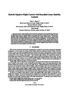
II. Adaptive Flight Control Consider the inner-loop adaptive flight control architecture shown in Fig. 1. The control architecture comprises: a reference model that translates rate commands into desired acceleration commands; a proportional-integral (PI) feedback control for rate stabilization and tracking; a dynamic inversion controller that computes actuator commands using desired acceleration commands; and a neural network direct MRAC with the optimal control modification.

Model Reference

1,

Y

PI Controller

I

+ x^

Dynamic Inversion

ar

Aircraft

X, u

Figure 1. Adaptive flight control architecture.

A. Adaptive Optimal Control Background Given a nonlinear plant as in Eq. (1) (t) = Ax (t) + B [ u (t )+f (x (t))] where x (t) : [0, o-) —^ R' is a state vector, it (t) : [0,—) —^ R P is a control vector, A E R"' and B E R n ' P are known such that the pair (A, B) is controllable, and f (x (t)) :118" --^ R P is a matched uncertainty. Assumption 1: The uncertainty f (x (t)) can be linearly parametrized using a set of basis functions in the form as shown in Eq. (2) ei* î (x (t )) + e (x (t )) = O*T4, (x ( t )) + e ( x ( t ))

f (x ( t ))

(2)

i=1

where O* E R " P is an unknown constant weight matrix that represents a parametric uncertainty, (D (x (t)) : R" —+ R" is a vector of known bounded basis functions that are continuous and differentiable in x, and e (x (t)) :118" --^ R P is an approximation error. The set of basis functions 4) (x (t)) is chosen such that the approximation error E (x (t)) is small such that JE (x (t))11 < co for all x (t) e -9 C R". The universal approximation theorem for sigmoidal neural networks by Cybenko can be used for selecting a good set of basis functions (D (x (t)). is Alternatively, Micchelli's theorem provides the theoretical basis for a neural network design of O T (t) CD (x (t)) using radial basis functions to keep the approximation error e (x (t) ) small. ) 5 The reference model is specified by Eq. (3) ^m

(t ) =

A m x,n ( t ) +B,n r ( t )

(3)

where a;" (t) : [0, 118" is a reference state vector, r(t) : [0, IEBr E y is a bounded piecewise continuous command vector, A", E R"" is Hurwitz, and B", E Ii8` with r < n. Since r (t) is bounded, x", (t) can be shown to be uniformly bounded such that Eq. (4): I x .. (0)11
A 22, B 1 ,

T

=A 11 x + A l2Z

+ B 1 u +,fl

and B2 are nominal undamaged plant matrices which are assumed to be known;

T

is a vector of roll, pitch, and yaw rates; z = [ Alb Aa AP AV Ah AB ] is a vector of perturbation in the bank angle A0, angle of attack Aa, sideslip angle A^ , airspeed AV, altitude A/1, and pitch angle

X = [ p q r ]


T

A0; it = [ A$„ ASe A5,. ] is a vector of additional aileron, elevator, and rudder deflections; and fi (r, z), i = 1, 2 is an uncertainty due to damage which can be approximated as shown in Eq. (18) *T

(18)

where cD (x,z) is a basis function chosen to be as shown in Eq. (19). (x, Z) =

r

XT pxT qxT

zT U T

rX

(x, z)

L

1T

(19)

J

The coupled basis function presented here is used to hopefully capture nonlinear error functions. If the damage response is highly nonlinear, then to model it accurately, a nonlinear function is a better fit than a simple linear function. The inner- loop rate feedback control is designed to improve aircraft rate response characteristics such as the shortperiod mode and the Dutch roll mode. A second-order reference model is specified to provide desired handling qualities with good damping and natural frequency characteristics as shown in Eqs. (20) through (22): 0,,,gp = slut (s +2y PwPS +cop)

z

y

(20)

= gg sror

(21)

( SZ +2^gcogs+wq ) Bm

( s2 +2^r(orS+C)r) / gym =

g r^ru,1

(22)

where 0,,,, 0,,,, and (3r„ are reference bank, pitch, and sideslip angles; cop , coq , and cor are the natural frequencies for desired handling qualities in the roll, pitch, and yaw axes; ^p, ^q , and are the desired damping ratios; 51at, 310r,, and Sriicl are the lateral stick input, longitudinal stick input, and rudder pedal input; and g p , g q , and g r are input gains. Let p,,, = O,,,, q,,, = 0,,,, and r,,, _ —(3,,, be the reference roll, pitch, and yaw rates. Then the reference model can be represented as shown in Eq. (23) .zm =

T where x,,, = L

pm q ,,, rm

],

— Kp xm —Ki r x„id-r+Gr fo

(23)

Kp = diag (2^po)p, 2^g cog , 2^r cor), Ki = diag (coy, O)q, cor ), G =diag (gp gg —gr ), and

T

r — [ 6I,R alorl Brad ] . Consider an optimal control allocation strategy when employing more control surfaces than the number of states to be controlled. Assuming the pair (A, I , B 1 ) is controllable and z is stabilizable, an angular rate feedback dynamic inversion controller is computed as shown in Eq. (24) 1

u, =B^ (BIBS )

K^

—

Kp + S'

a`+Gr—A 11 x— Al2z —O T (24)

where u, is a control surface deflection command vector. Note the pseudo -inverse required when B 1 is non-square. T

Let e = [ fo (x,,, —x)d r equation is given by Eq. (25)

x,,, —x ]

be the tracking error and set the input gains to one, then the tracking error

(25)

e=A,,,e+B(Oi—s^ where Eqs. (26) and (27) A,n =

0

1

(26)

—K1 —KI,

B= ^ 0

(27)

Let Q = 21, then the solution of the Lyapunov equation, Eq. ( 11), yields Eq. (28). (K`+1) P— K` 1Kp+KP1 KA 1

K' 1 KP 1 (1 + K,— 1)

5 of 17

American Institute of Aeronautics and Astronautics

>0

(28)

An, 1 is computed to be Eq. (29). -1

A in —

—Ki K, —K; I 1

I

0

(29)

Evaluating the term BT PA —n 1 B of the adaptive law shown in Eq. (10) yields Eq. (30). BT PAn, 1 B = —K,— '

G

0

(30)

Finally, applying the adaptive optimal control modification, the weight update law is then given by Eq. (31). 0 1 = — F(D (eTPB+v(DT 0 1 Ki `)

(31)

Changing v affects the damping of the closed loop response and will be shown in the results section.

III. Simulation Results for F-18 Aircraft Model To test an adaptive system, a failure needs to be simulated; however, in the "real world" the failure will not be known or at best can be isolated to a subsystem. Most failures are typically covered by aerodynamic failures or control effectors malfunctions. A "real world" failure is a shift in the center of gravity (cg) and is presented below. A control surface failure is another "real world" type of failure. The cont rol failure that is shown in this paper is for illustration purposes and is not intended to represent a true failure. This section presents results from simulations of [A] matrix and [B] matrix failures. An aerodynamic type of failure [A] is inserted first with a large cg aft shift, this corresponds to a change in C,,,x . The second type of simulated failure, which represents a surface failure, inserts a jammed left stabilator, which is the [B] matrix failure. Results from the simulation runs are presented to illustrate the advantages of adaptation compared to the baseline dynamic inversion without adaptation. The flight condition used in this paper is a test point of Mach 0.5 and an altitude of 15,000 ft. All of the pilot inputs to the simulation time histories are from "canned" piloted stick inputs and no attempt to correct for the aircraft attitudes are added to the piloted inputs. This "canned pilot input" method was used only for comparison purposes. For instance, when a failure is imparted on the aircraft and the resulting attitudes change minimally, the control system is said to have good restoring properties. All the test cases have a one frame delay (1/100 second) at the actuators for added realistic implementation purposes. This delay may not be adequate for some designs. A. [A] Matrix Failure (Aerodynamic Type Failure) The first case is an [A] matrix failure imposed on the aircraft with a destabilizing cg shift or a C,,, a change. Figure 2 shows a 40-second time history in which 3 longitudinal pilot stick inputs are presented and the failure is imposed at 13 seconds. In the first 13 seconds a normal health response shows how the pitch rate follows the commanded pitch rate (green) and the stick command (black). After the failure is inserted, the response without adaptation shows that the aircraft is stable but with low damping and 2 overshoots (blue). With adaptation on (red), the response is much better and follows the commanded pitch rate. By the third pilot input, the adaptation response is close to the commanded pitch rate. Notice the low tracking error between q ref and q before the failure and the better tracking response with adaptation after the failure. Figure 2 also shows the angle of attack and normal acceleration responses associated with the C,,, a change; and that the system behaves better with adaptation than without. Figure 3 shows the tracking error in the roll, pitch and yaw axes along with the adaptation weights. The errors are better with adaptation and the weights are convergent. The results show that the adaptation helps with respect to the tracking task (q command) and increases the damping. Figure 4 shows the surface positions with and without adaptation. The actuator models are high-fidelity fourthorder models with time delays. As expected, the surfaces are well-damped with adaptation on. After observing the weights and how they converge, the control surfaces, and the tracking errors, the final analysis for the [A] matrix failure example shows that adaptation helps compared to the no adaptation case.


LU

15 10 5 Q 0 -5 -10 -15 20 0

5

10

15

20

25

30

35

40

0

5

10

15

20

25

30

35

40

0

5

10

15

20

25

30

35

40

20 15 a

10

a

5 0 -5 -10

1 0.5 0

0

ac -0.5 -1 15

Time, s

Figure 2. Time history of longitudinal states due to an [A] matrix failure C., shift at 13 seconds with and without adaptation.

0.02

0.01

.°

-0.01

-0.02-0.03

^-`^

0

^^^ --^- - ----'

^/- -\-^ _-^---^-i' /

_ _ _ p err Adap perr No Adap

i

5

10

15

20

25

15 10

30

..

i

40

- gerr Adap -' - q err No Adap

\

0 ——————————— ————— d -5 Q -10 -

35

-15 0

5

10

15

20

25

30

35

40

5 /"

\.

^

0

-

—— — —

rerr Adap

rerr No Adap

-5 0

5

10

15

20

25

30

35

40

25

30

35

40

Time, s a n i5

0.06 0.04 0.02 0

C -0.02 3 -0.040

5

10

15

20

Figure 3. Time history of tracking errors due to an [A] matrix failure C., shift at 13 seconds with and without adaptation.


0.1

0.050

^^

- - - Ail Adap

- . - - Ail No Ada

lip -`^.

^'`

--

â -0.05 -0.1 0

5

10

15

20

25

30

35

40

3

2

,

N 1

j

`\

-2

- - -

-

Stab Adap

• - • Stab No Adap

5

10

15

20

25

30

35

40

3

2a 1 0—

J

\

_ 0

rn

.

-.

î ^'\

^.-. ,

i

i ^'

- - - L satb Adap - - L stab No Adap

\

T

V.

_2 0

5

10

15

20

25

5

30

35

40

^.\ - - - Rud Adap -- -- RudNoAdap

N \

-5

^. 2

-10 0

5

10

15

20

25

30

35

40

Time, s Figure 4. Time history of control su rfaces due to an [A] matrix failure C,,,. shift at 13 seconds with and without adaptation.

B. [B] Matrix Failure (Control Surface Januned) The second case is a [B] matrix failure imposed on the left stabilator 13 seconds into the simulation run. The left stabilator is jammed (or locked) at +2.5 degrees from trim. Figure 5 shows a 40-second time history of the longitudinal responses. During the first 13 seconds the pitch rate follows the commanded pitch rate, but after the failure insertion there is a large downward motion and the system cannot track very well. Aircraft response comparison with this [B] matrix failure shown in Fig. 5 indicates a better response with adaptation on. Pitch rate follows the reference better with adaptation on. The lateral-directional responses from the same longitudinal command also show better aircraft response with adaptation, as shown in Fig. 6. The roll rate with adaptation is smaller than without adaptation. The bank angle and sideslip angle both come back to wings-level with adaptation but stay at 10 degrees and 8 degrees, respectively, without adaptation. Note that there are no lateraldirectional pilot inputs (p1e f , r1e f are zero). Figure 7 shows smaller tracking errors and converging neural networks weights. Analysis indicates the system is stable and the performance is better with adaption.


4 2 a 0 a d -2 a -4 -6 8 0

5

10

15

20

25

30

35

40

10

8

/

6 -^

- - - a Adap - - a No Adap

i

1

4--

0-2 0

5

10

15

0

5

10

15

20

25

30

35

40

20

25

30

35

40

0.8 0.6 0.4 0.2 0

-0.2 -0.4 -0.6 08

Time, s

Figure 5. Time history of longitudinal states clue to a [B] matrix failure (stabilator jammed at 2.5 degrees at 13 seconds with and without adaptation.

IS

10 5 0

n

CL -5N, -15r_.^ 0

5

10

15

20

25

30

35

40

30

20 °0 10 0 --- — ---- -- _. _10

0

5

10

--- - -ONoAdap

__-_- 15

20

25

30

35

40

0.5

0

---

--- -^\-

---7,

--— \

j

L ---

--^^

^ ,'

J ? -0.5

--- rAdap - - r No Adap

_1 0

5

10

15

20

25

30

35

40

10

°1 0

------

4

No Map

a 2 -2 0

5

10

15

20

25

30

35

40

Time, s

Figure 6. Time history of lateral/directional states due to a [B] matrix failure (stabilator jammed at 2.5 degrees at 13 seconds with and without adaptation.


iu 5 'a 0 -5 -10 15

0

5

10

15

20

25

30

35

40

8 42 4

q.,Adap / - - _ q., No Adap ^^ ii '

a

2

-

• -

T 0 -2-

0

5

10

15

0

5

10

15

20

25

30

35

40

20

25

30

35

40

25

30

35

40

1 a

0.5 0 05

Time, s

n 4 a 3 2 `^

1

0 0 -2

0

5

10

15

20

Figure 7. Tune history of tracking errors due to a [B] matrix failure (stabilator jammed at 2.5 degrees at 13 seconds with and without adaptation.

C. [A] Matrix Failure for Variable Learning Rate (n and Damping (v) Test Cases This section shows the adaptation rate gamma (F) can be increased and the aircraft will remain stable. This optimal control modification method enables fast adaptation with good damping. The test case changes the adaptation rate from 0.5 to 50 while keeping the damping term (v) constant at 1. Figure 8 shows the same [A] matrix failure as that presented in subsection A, but the failure shown in Fig. 8 occurs at 2 seconds instead of at 13 seconds and is followed by a pitch input. As Fig. 8 shows, the pitch rate tracking error is large with a F of 0.5 compared to 50. The weights are also shown, and the larger adaptation rate increases the size of the weights as expected. Note that in both cases the system weights are convergent and the tracking error is better with the larger adaptation rate. Figure 9 shows what happens when the damping term is changed (v from 0.25 to 1) while keeping the adaptation rate constant (F = 5). The tracking error has low damping with the lower v term of 0.25 as expected. In both cases the weights converge to reasonable values. The results and analysis show that larger adaptation rates can be tolerated with this optimal control modification technique. The dalnping term can be used to tune the desired performance.

10 of 17


10

gerr With High Gain r' gerr With Low Gain r \

r

5 at v

0

/

\

i

5 0

5

10

15

0.5 0.4

Wts With High Gain r - • - Wts With Low Gain r'

r

n 0.3 4/

Q 0.2

///ter—-------------------------^

rn 0.1

/

0

—=t==——------------------

-0.1 02 0

5

10

15

Time, s Figure 8. Time history of pitch rate error and weights due to an [A] matrix failure C

at 2 seconds; learning rate F of 0.5 and 50 with

fixed damping term v = 1.

10

gerr High v

/

-

-

-•- %, Low v W

5

42

r

a

u 0

/

—5J L 0

J

I

5

10

15

0.3

Wts High v Wts Low v

0.2 n 0.1

am

0

L rn -0.1 `r

-0.2 -0.3

04 0

5

10

15

Time, s

Figure 9. Time history of pitch rate error and weights due to an [A] matrix failure C m , shift at 2 seconds; fixed learning rate F = 5 and variable damping term v of 0.25 and 1.

IV. Conclusions This study presents a new modification to the standard model-reference adaptive control based on an optimal control formulation of minimizing the Y2 norm of the tracking error. The optimal control modification adds a damping


term to the adaptive law that is proportional to the persistent excitation. The modification enables fast adaptation without sacrificing robustness. The modification can be tuned using a parameter v to provide a trade-off between tracking performance and damping. Increasing v improves damping to unmodeled dynamics. Simulations of a damaged F-18 aircraft showed improvements in performance when compared to the baseline controller. V. Appendix Given a nonlinear plant as in Eq. (32)

x(t) = Ax (t) + B [u (t) + f (x (t))]

(32)

where x (t) : [0,—) ---^ 118" is a state vector, it(t) : [0,—) —^ R P is a control vector, A E R" I and B E R" P are known such that the pair (A, B) is controllable, and f (x (t)) :1[8" —^ R P is a matched uncertainty. Assumption: The uncertainty f (x (t)) can be linearly parametrized using a set of basis functions in the form as Eq. (33)

f (x (t ))

8^* 4a (x (t )) + E (x (t )) = O*T4' (x ( t )) + ( x ( t ))

(33)

where O* E II8` P is an unknown constant weight matrix that represents a parametric uncertainty, (D (r (t)) : R' —+1[8'" is a vector of known bounded basis functions that are continuous and differentiable in x, and E (x (t)) :1[8" —+ R P is an approximation error. The set of basis functions 4) (x (t)) is chosen such that the approximation error E (x (t)) is small such that 11E (x (t)) II < co for all x (t) E _9 C 118". The universal approximation theorem for sigmoidal neural networks by Cybenko can be used for selecting a good set of basis functions (D (x (t))." Alternatively, Micchelli's theorem provides the theoretical basis for a neural network design of O T (t) (D (x (t)) using radial basis functions to keep the approximation error E (x (t) ) small.'5 The reference model is specified by Eq. (34) _tm ( t )

= Amxm ( t ) + B, " r ( t )

(34)

where x,,, (t) : [0,—) —^ R" is a reference state vector, r(t) : [0,—) --^ R' E Y is a bounded piecewise continuous command vector, A", E R""" is Hurwitz, and B", E R"" with r < n. Since r (t) is bounded, x ", (t) can be shown to be uniformly bounded such that Eq. (35).

Ix, " (0) II < e ==^, II x ", (t) II 0

(35)

The objective is to design a full-state feedback adaptive control to enable x (t) to follow x ", (t) with the controller shown in Eq. (36) u (t) = Kxx (t) +K, r (t) — tt d (t) (36) where Kx E RP " and K,- E RP "' are gain matrices and parametric uncertainty in the plant such that Eq. (37)

u,„ t (t)

E R P is a direct adaptive signal which estimates the

1W ( t ) = OT ( t ) ,' ( x (t))

(37)

where O (t) E lE8` P is an estimate of the parametric uncertainty W. Assumption 2: There exist K; and Kr such that the model matching conditions shown in Eqs. (38) and (39) are satisfied. Am =A + BKx B ", = BKr

(38) (39)

Let O (t) = O (t) — O* be an estimation error of the parametric uncertainty and define the tracking error as e (t) x,,, (t) —x (t), then the tracking error equation becomes Eq. (40). e (t) = A,,,e (t) +B IOT (t) (D (x (t)) — E (x (t))1

(40)

Proposition : The adaptive law shown in Eq. (41) provides an update law that minimizes Il e (t) lly2 o (t) _ -rte

(x (t)) 1 T (t) P - VCDT (x (t)) O (t) BT PA;" ' B 12 of 17


(41)

where I' = rT > 0 c R"' x "' is an adaptive gain matrix, v > 0 c R is a weighting constant, and P = P T > 0 c ][3"x" solves Eq. (42) (42) PA,,, +A,TP = -- where Q = Q T > 0 E R"x" Proof: The adaptive law seeks to minimize an infinite-time horizon cost function as Eq. (43) r

J= line 1 ^t [e(t)-0(t)]T Q [e (t) — A (t)] dt tf ^^^ 2 a

(43)

subject to Eq. (40) where A represents the unknown lower bound of the tracking er r or shown in Figure 10.

Figure 10. Tracking error lower bound.

J is convex and represents the distance measured from the normal surface of a ball Br C -9 C R n with a radius A. The cost function is designed to provide robustness by not seeking the tracking error that tends to zero but rather to some lower bound away from the origin. By not requiring e (t) -4 0 as t -4 —, the adaptation can be made to be robust. Therefore, the tracking performance can be traded with robustness by a suitable selection of the tuning parameter v. This optimal control problem can be formulated by the Pontryagin's Minimum Principle. Defining a Hamiltonian, Eq. (44),

H(e(t),o(t))

=

I[e(t)—o(t)]TQ[e(t)—o(t)] + PT (t)[A",e(t)+BOT(t)41(x(t))—B£(a(t))] (44)

where p (t) : [0,00) -4 R' is an adjoint variable, then the necessary condition gives Eq. (45)

(45)

)5 (t) = —VHe = —Q [ e ( t ) — A(t)] — Amp (t)

with the transversality condition p ( tf -+ oo) = 0 since e (0) is known. The adaptive law can then be formulated by a gradient update law as Eq. (46). O(t) _ —FVHOT = —DD(v(t))OHGT(D _ —T('(x(t))PT (t ) B

(46)

The solution of p (t) can be obtained using a "sweeping' method by letting p (t) = P (t) e (t) +S (t) O T (t) CD (x (t)). Then, Eq. (47)

P(t)e(t)+P(t) (A",e(t)+BOT (t)4D.(.r(t))— BE) *TCD(X(t))—B£(r(t))) +S(t)O T (t)^(.x(t)) +S(t)

d (O

T

(t)CD(a(t))) =—Q[e(t)—A(t)]

-A ,T ^P(t)e(t)+S(t)OT

which yields Eqs. (48) through (50)

P(t)+P(t)An,+Ain (t) +Q=0 S(t)+P(t)B+A„T,S(t) =0

QA (t)—

S (t) d(O

T

(t)CD(X(t)))

+P(t)BIO*T(D(X(t))+£(x(t))I=0


(t) CD

(47)

(48) (49) (50)

subject to the transversality conditions P (t f —+ -) = 0 and S (t f —^ -) = 0. Introducing a time-to-go variable r = t f — t, then the Lyapunov differential equation shown in Eq. (48) becomes Eq. (51) dP (51) +P(z)Ain+A,Tn P(i)+Q=0

d-r

subject to the initial conditions in time-to-go P(0) = 0, for which the existence and uniqueness of its solution is well-established. It follows that Eq. (49) also has a stable, unique solution in time-to-go since A n, is Hurwitz, Eq. (52),

dr —

+P(T)B+A'S(z)=0

(52)

subject to S (0) = 0. The solutions of P (z) and S (r) as r —^ oo approach to their steady-state solutions as shown in Eqs. (53) and (54). PA m +AmP = —Q

(53)

S = —A in PB

(54)

Without any loss of generality, a weighting constant v > 0 E R is introduced as a gain to allow for adjustments of the modification term in the adaptive law, where v = 1 corresponds to an optimal solution. Thus, Eq. (55). S= —vA in—T PB

(55)

The adjoint p is then obtained as shown in Eq. (56). p (t) = Pe (t) — vAm T PBO T (t) (D (x (t))

(56)

Since O* is constant, it follows that the adaptive law, shown in Eq. (41) 5 is obtained from Eqs. (46) and (56). Theorem: The adaptive law shown in Eq. (41) results in stable and uniformly ultimately bounded tracking error e (t) for all (e (0) ,O (0)) E 111p with an ultimate bound as shown in Eq. (57) P

_

X,.,x (P) ^2 +^m'. (T-1 ) K`

(57)

/min (P)

where Eqs. (58) and (59) _

2PBe Xmin (Q)

(5$)

K = 2IIBTPA—'BII Oo Amin ( BT A nt i QA,-,'B)

(59)

with Eo = sup, 11E (t)11 and Oo = I1O * 11.

Proof: Choose a Lyapunov candidate function as shown in Eq. (60).

V (t) = e (t)Pe (t) +trace (O T (t) F -1 O (t))

(60)

Evaluating V yields Eq. (61).

^(t)=eT (t) (A,,,P + PA,n) e (t) + 2e T (t)PBIO T (t) p(x(t))—E(a(t))] —2trace(O T (t)^(x(t)) le T (t)PB—v^ T (x(t))O(t)B T PA inn 'BI ) (61) Using the trace identity trace (A T B) =BA T , V (t) can be written as shown in Eq. (62).

T

V (t) _ —eT (t) Qe (t) + 2eT (t) PB IO (t) q) (x (t)) — e (x (t) )] — 2e (t) PBO T (t) CD (x (t)) +2 V(pT (x (t)) O (t) BT PA —n 1 BOT (t) 4) (x (t)) (62) 14 of 17 American Institute of Aeronautics and Astronautics

The sign-definiteness of the term PAn, is now considered. Recall that a general real matrix G is positive ( negative) definite if and only if its symmetric part G = 2' (G+GT ) is also positive (negative) definite. Then, by pre- and postmultiplication of Eq. (42) by AmT and A„', respectively, PA,—n 1 can be decomposed into a symmetric part M and anti-symmetric part N as shown in Eq. (63) (63)

PA—n' =M+N

where Eqs. ( 64) and (65) M=— (Am T P+PA n,') 2 N

2

(PA — '

= --A)- QA_

(64)

(65)

—A in P) .

Since the symmetric part M < 0, then PA —n 1 < 0. Thus, V (t) becomes Eq. (66).

V ( t ) =—eT ( t ) Qe ( t ) - 2eT (t)PBE(.1:(t))—VAT (x ( t ) ) O ( t ) BTA m T QA m' BOT (t)^(\:(t)) +2V4) T (x(t))0(t)B T NBO T (t) cD (x (t)) + 2V(DT (x (t)) O*BTPA ," 1BOT (t)4)(x(t)) (66) Letting y (t) = BO T reduced to Eq. (67)

(t) cD (x (t)) and using the property yT (t)Ny (t) = 0 for an anti-symmetric matrix N, V (t) is

V =—e T (t)Qe(t)-2e T (t)PB£(x(t))— V(DT (x(t))6(t)B TA —T QA n,'BO T (t)Cp(x(t)) +2v CD T (r(t))O*B T PA n 'BO T (t)0(x(t)) (67)

which is bounded by Eq. (68).

V (t) 0 ^(x(t))e T (t)PB+µ IleT (t)PB I 10(t) , u > 0 0(t) = —1 cD(x(t))eT (t)PB—v4)T (x(t))0(t)BTPAM'B , v > 0

Optimal

Table 1. Modifications to model-reference adaptive law. The lack of robustness was well studiedl', I`l and subsequently motivated the development of the 6- modification] and e-modification. 11,20,21 In this context, the parameter v plays the same role as the parameters 6 in the 6- modification andµ in the e-modification that provides a trade-off between tracking performance and stability robustness. Thus, v has to be selected small enough to provide a desired tracking performance, but large enough to provide sufficient robustness against time delay or unmodeled dynamics.

References I Burken, John, Curtis Hanson, James Lee, John Kane shige, "Flight Test Comparison of Different Adaptive Augmentations of Fault Tolerant Control Laws for a Modified F-15 Aircraft ", AIAA Infotech@Aerospace Conference, AIAA-2009-2056. 2Steinberg, M. L., "A Comparison of Intelligent, Adaptive, and Nonlinear Flight Control Laws', AIAA Guidance, Navigation, and Control Conference, AIAA-1999-4044, 1999. 3 Eberhart, R. L. and Ward, D. G., "Indirect Adaptive Flight Control System Interactions', International Journal of Robust and Nonlinear Control, Vol. 9, pp. 1013-1031, 1999. 4Rysdyk, R. T. and Calise, A. J., "Fault Tolerant Flight Control via Adaptive Neural Network Augmentation", AIAA Guidance, Navigation, and Control Conference, AIAA-1998-4483, 1998. 5 Kim, B. S. and Calise, A. J., "Nonlinear Flight Control Using Neural Networks', Journal of Guidance, Control, and Dynamics, Vol. 20, No. 1, pp. 26-33, 1997. 6Johnson, E. N., Calise, A. J., El-Shirbiny, H. A., and Rysdyk, R. T., "Feedback Linearization with Neural Network Augmentation Applied to X-33 Attitude Control', AIAA Guidance, Navigation, and Control Conference, AIAA-2000-4157, 2000. 7 Idan, M., Johnson, M. D., and Calise, A. J., "A Hierarchical Approach to Adaptive Control for Improved Flight Safety", AIAA Journal of Guidance, Control and Dynamics, Vol. 25, No. 6, pp. 1012-1020, 2002. 8 Hovakimyan, N., Kim, N., Calise, A. J., Prasad, J. V. R., and Corban, E. J., "Adaptive Output Feedback for High-Bandwidth Control of an Unmanned Helicopter", AIAA Guidance, Navigation and Control Conference, AIAA-2001-4181, 2001. 9Cao, C. and Hovakimyan, N., "Design and Analysis of a Novel LI Adaptive Control Architecture with Guaranteed Transient Performance". IEEE Transactions on Automatic Control, Vol. 53, No. 2, pp. 586-591, 2008. ' O N. Nguyen, K. Krishnakumar, J. Kaneshige, and P. Nespeca, "Flight Dynamics and Hybrid Adaptive Control of Damaged Aircraft", AIAA Journal of Guidance, Control, and Dynamics, Vol. 31, No. 3, pp. :751-764, 2008. 11 Slotine, J.-J. and Li, W., Applied Nonlinear Control, Prentice-Hall, 1991. 12 loannu, P.A. and Sun, J., Robust Adaptive Control, Prentice-Hall, 1996. 13 Nguyen, N., Krishnakumar, K., and Boskovic, J., "An Optimal Control Modification to Model-Reference Adaptive Control for FastAdaptation", AIAA Guidance, Navigation, and Control Conference, AIAA 2008-7283, 2008. 14Cybenko, G., "Approximation by Superpositions of a Sigmoidal Function", Mathematics of Control Signals Systems, Vol. 2, pp. 303-314, 1989. 15 Micchelli, C. A., "Interpolation of Scattered Data: Distance Matrices and Conditionally Positive Definite Functions", Constructive Approximation, Vol.2, pp. 11-12, 1986.


16 1(halil, H.K. Nonlinear Systems, Princeton-Hall 2002. 17 Narendra, K. S. and Annaswamy, A. M., A New Adaptive Law for Robust Adaptation Without Persistent Excitation', IEEE Transactions on Automatic Control, Vol. AC-32, No. 2, pp. 134-145, 1987. 18Rohrs, C.E., Valavani, L.. Athans, M., and Stein, G., "Robustness of Continuous-Time Adaptive Control Algorithms in the Presence of Unmodeled Dynamics". IEEE Transactions on Automatic Control, Vol AC-30, No. 9, pp. 881-889, 1985. 19Jacklin, S. A., Schumann, J. M., Gupta, P. P., Richard, R., Guenther, K., and Soares, F., "Development of Advanced Verification and Validation Procedures and Tools for the Certification of Learning Systems in Aerospace Applications", AIAA Infotech @ Aerospace Conference. AIAA-2005-6912, 2005. 20 Bryson, A.E. and Ho, Y.C., Applied Optimal Control: Optimization, Estimation, and Control, John Wiley & Sons Inc., 1979. 21 Nguyen, N., and Jacklin, S., "Neural Net Adaptive Flight Control Stability, Verification and Validation Challenges, and Future Research', Workshop on Àpplications of Neural Networks in High Assurance Systems", International Joint Conference on Neural Networks, 2007.


Can Modern Control Systems Help the Pilot Out Even More Than Traditional Methods????

   

The above were survivable accidents; Can Adaptation help more. Objectives ◦  Regain a Stable Platform   Evaluate Robustness metrics for nonlinear adaptive systems ◦  Maneuverability (can you fly it around)   Control vehicle within new constraints / structural loads etc.. ◦  Provide the ability to safely land the airplane   Develop safest recovery trajectory

Given a nonlinear plant

Assumption1 : The uncertain f(x(t)) can be parameterized using a basis function in the following form.

Θ  is a unknown weight matrix / Θ  Φ is a vector of known bounded basis functions (continuous & differentiable in x) ε  is an approximation error The reference model is: Since r(t) is bounded, xm can be shown to be uniformly bounded such that:

The objective is design a feedback adaptive control to enable x(t) to follow

Assumption2 : There exist Kx & Kr such that the model matching conditions shown below are satisfied.

e(t) = xm(t) – x(t)

The adaptive law:

(1)

Ioannu

(2)

Narendra and Annaswamy

Z

t

x_d = A m x m + B m r + K p ( x m ¡ x ) + K i ( x m ¡ x ) d¿ ¡ ua d 0 ¡ 2 2 2¢ K p = di ag ! 1 ; ! 2 ; ! 3 ; K i = di ag ( 2»1 ! 1 ; 2»2 ! 2 ; 2»3 ! 3 ) !

1 »i = p 2

i

u = B¡

1

( x_d ¡ A x ¡ B u ¡ Gz)

Transient Performance

MRAC

°

º

Stability Robustness

º

Optimal Control Modification

[A] matrix failure: CG shift @ 13 seconds

[A] matrix failure: CG shift @ 13 seconds

[B] matrix failure: Left stabilator jammed at 2.5 deg @ 13 seconds

[B] matrix failure: Left stabilator jammed at 2.5 deg @ 13 seconds

Adaptation rate change from .5 to 50. with a shift in CG at 2 seconds