doi: 10.5028/jatm.v8i2.608
Formation Flight Control of Multi-UAV System with Communication Constraints Ruibin Xue1, Gaohua Cai2
Abstract: Three dimensional formation control problem of multi-UAV system with communication constraints of non-uniform time delays and jointly-connected topologies is investigated. No explicit leader exists in the formation team, and, therefore, a consensus-based distributed formation control protocol which requires only the local neighbor-toneighbor information between the UAVs is proposed for the system. The stability analysis of the proposed formation control protocol is also performed. The research suggests that, when the time delay, communication topology, and control protocol satisfy the stability condition, the formation control protocol will guide the multi-UAV system to asymptotically converge to the desired velocity and shape the expected formation team, respectively. Numerical simulations verify the effectiveness of the formation control system. Keywords: Three dimensional formation control, Jointly-connected topologies, Multi-UAV system, Non-uniform time delays, Consensus protocol.
Introduction Recently, with the development of computer control, sensors, communication network etc., many researches on the formation flight control have been performed. This is because various missions can be successfully completed by the formation flight, such as battlefield reconnaissance, multi-target attacking, environment monitoring and earthquake rescue and so on. Multi-UAV coordinated formation control has overwhelming superiority in high efficiency in performing tasks, low cost of fuel, strong robustness and more flexibility compared with single UAV (Ren and Beard 2008; Cao et al. 2012). Therefore, multi-UAV formation flight control has become a hot topic in UAV field. In earlier years, typical approaches for formation control could be roughly categorized as leader-follower, behavioral, virtual leader/virtual structure. Most of the formation flight researches are performed based on the leader-follower approach, where some UAVs are designed as leaders while others are designed as followers (Ren 2007; Giulietti et al. 2000). In this approach, the leaders track the predefined trajectory, and the followers track the nearest leaders according to given schemes. It is easy to analyze and implement the leader-follower controller. However, the leader is a single point for the formation, and therefore this approach is not robust with respect to the leader failure. In recent years, the problem of multi-UAV cooperative formation flight control based on consensus protocol has drawn substantial research effort from many studies (Kuriki and Namerikawa 2013; Menon 1989; Ren 2006; Seo et al. 2012). Ren (2007) extended a consensus protocol, which is introduced for systems modelled by second-order dynamics, to tackle multi-UAV formation control problems by appropriately choosing information states on which consensus is reached. Seo (2009)
1.Beijing Institute of Technology – School of Aerospace Engineering – Key Laboratory of Dynamics and Control of Flight Vehicle – Beijing – China. 2.Beijing Aerospace Automatic Control Institute – Beijing – China. Author for correspondence: Ruibin Xue | Beijing Institute of Technology – School of Aerospace Engineering | Tiyu N Rd, Haidian | Beijing – China | Email:
[email protected] Received: 01/25/2016 | Accepted: 04/26/2016
J. Aerosp. Technol. Manag., São José dos Campos, Vol.8, No 2, pp.203-210, Apr.-Jun., 2016
204
Xue R, Cai G
proposed a consensus-based formation flight control protocol and proved that the multi-UAV system can form and maintain a geometric formation flight with the network topology switching between a directed strongly-connected topology and a topology with a spanning tree. Dong et al. (2014) investigated the timevarying formation control problem by applying a consensus-based formation control protocol, and necessary and sufficient conditions are obtained for the stability of the system which contains a spanning tree in the fixed topology. Then a quadrotor formation platform was introduced to validate the theoretical results. However, most of the researches about consensus-based cooperative formation flight control are mainly focused on two systems: one is a fixed communication topology without time delays; the other is a switching communication topology without time delays as well. There are few results available to treat the formation control system with jointly-connected topologies and time delay. But, in reality, the time delay usually exists due to transmission rate and network congestion, and the communication topology of the multi-UAV system will be changed owing to communication jamming, complex terrain, limitation of communication distance etc. Therefore, it is of great significance in both theory and application to investigate cooperative formation flight control by considering time delay and changing topology. The main contributions of the paper can be summarized as follows. First, to design a new formation flight control protocol considering two key-problems: one is the diverse and asymmetric time delays, and the other is the dynamically changing topologies. The topologies discussed here may not connect all the time but the union of the topologies is connected in each period of time. Second, the analysis of the complex topologies is turned to a simple research of connected component in each period of time according to the stability analysis, and a sufficient condition for the stability is obtained based on Lyapunov theory. The multi-UAV system can shape and maintain the expected formation with desired velocity, when it satisfies the sufficient condition.
Model of the multi-UAV system This paper considers a group system consisting of n autonomous UAVs, and the point-mass model is used to describe the motion of the UAV formation flying. The related variables are defined with respect to the inertial coordinate system and are shown in Fig. 1 (Wang and Xin 2012).
Local vertical
h ϕ
V
Vertical plane
T-D 0
γ
L
y Horizontal plane
χ x
T-D: Thrust-drag; χ: Heading angle; L: Lift; g: Flight path angle; V: Ground speed; ϕ: Banking angle.
Figure 1. UAV model.
The model assumes that the aircraft thrust is directed along the velocity vector and that the aircraft always performs coordinated maneuvers. It is also assumed that the Earth is flat, and the fuel expenditure is negligible, i.e. the center of mass is time-invariant (Xu 2009). Under these assumptions, the motion equations of the ith UAV can be described as follows:
(1)
where: i = 1, 2, …, n is the index of multiple UAVs under consideration. For UAVi, xi is the down-range; yi is the cross range; hi is the altitude; vi is the ground speed; γi is the flight path angle; χi is the heading angle; Ti is the engine thrust; Di is the drag; mi is the mass; g is the acceleration due to gravity; ϕi is the banking angle; Li is the vehicle lift. The control variables in the UAVs are the g-load ni = Li/gmi, controlled by the elevator, the banking angle ϕi, controlled by the combination of rudder and ailerons, and the engine thrust Ti , controlled by the throttle. Throughout the formation control process, the control variables will be constrained to remain within their respective limits. Define Rm × n as a m × n real matrix set, ξi = [xi ,yi ,hi]T ∈ R3, . . . and ui = [uxi ,uyi ,uhi]T ∈ R3. Differentiating vi ,γi ,hi with respect to time twice and substituting xi ,yi ,χi , one has the transformed dynamic models of the ith UAV as follows:
J. Aerosp. Technol. Manag., São José dos Campos, Vol.8, No 2, pp.203-210, Apr.-Jun., 2016
(2)
where: ξi is the position of UAVi ; ui is a new control variable,
Formation Flight Control of Multi-UAV System with Communication Constraints
and the relationship between ui and the actual control variable Ui is given by the expressions (Xu 2009): (3)
(4)
(5)
Formation control protocol design of the multi-UAV system The multi-UAV system and its behavior are described in graph theory. It is supposed that the multi-UAV system under consideration consists of n UAVs and G(Γ, E, A) is an undirected graph of the multi-UAV system, where Γ = {s1, s2, …, sn} is the set of nodes, ℓ = (1, 2, 3, ..., n) is the set of the number of nodes, and E = {(si ,sj) ∈ Γ × Γ, i ≠ j} is the set of edges. At each time, each UAV updates its current state based upon the information received from its neighbors. Undirected graphs are used to model communication topologies. Each UAV is regarded as a node. Each edge (si , sj) or (sj ,si) corresponds to an available information link between UAVi and UAVj. A communication topology is formed when the UAVs begin to communicate to each other at any time. In reality, the communication topology usually switches due to link failure brought by communication blocking, external disturbance, hardware failure etc. To describe the variable topologies, a piecewise constant switching function σ(t): [0, ∞ → p = {1, 2, ..., N}(σ in short) is defined, where N denotes the total number of all possible communication undirected graphs. The communication graph at time t is denoted by Gσ and the corresponding Laplacian, by Lσ. This paper investigates the design of the control protocol of the multi-UAV system under jointly-connected communication graph. The state-space form of the dynamics of the ith UAV is obtained from Eq. 2, as follows:
205
We say that the control protocol ui (t) solves the formation control problem if the states of UAVs satisfy lim [ξi (t ) – ξj (t)] = rij t=→+∞ and lim ζi (t ) = ζi (t ) = ζ* (rij = −rji is the expect distance between t=→+∞ UAVi and UAVj in formation and ζ* ∈ R3 is the expect velocity), i.e. the multi-UAV system can shape and maintain an expected formation with a desired velocity under the control protocol ui(t). In this paper, a formation flight control protocol for the multi-UAV system is designed, and the two key-problems of non-uniform time delays and jointly-connected topologies are considered. To solve this problem, a linear control protocol for the ith UAV is firstly presented, as follows:
(7)
(6)
where: aij(t) is the adjacency weight of the communication graph Gσ ; Ni(t) is the neighbor set of the ith UAV; k1 > 0, k2 > 0, and k3 = k1k2; τii(t) is the time-varying self-delay of the ith UAV that may be caused by measurement or computation, and τij(t) is the time-varying delay for the ith UAV to get the state information of the jth UAV. Here, it is not required that τij(t) = τji(t). It is supposed that there are altogether M different time delays, denoted by τm(t) ∈ {τii(t), τij(t), i, j, ∈ ℓ), m = 1, 2, …, M, satisfying the following assumptions 1 and 2. Assumption 1: the time-varying delays τm(t), m = 1, 2, …, . M (τm in short), satisfy 0 ≤ τm(t) ≤ hm and τm(t) ≤ dm < 1 for specified constants hm > 0 and dm > 0. A model transformation is made to analyze the close-loop control performance of the multi-UAV system. Therefore, the concept of formation center is introduced, which is a formation centroid of the multi-UAV system. A formation of “regular pentagon” is considered as an example for convenient and easy understanding of the formation problem, as shown in Fig. 2, where O is the origin of Cartesian coordinates, OC is the formation center, ξi(t) and ξj(t) are positions of UAVi,j in plane coordinate system, respectively, and ξ0(t) is the formation center. The distance between UAVi,j and the formation center are ri and rj , respectively. Consequently, the control protocol (Eq. 7) can be transformed into:
where: ξi (t) ∈ R3 is the position state; ζi (t) ∈ R3 is the velocity state; ui (t) ∈ R3 is the control input.
(8)
J. Aerosp. Technol. Manag., São José dos Campos, Vol.8, No 2, pp.203-210, Apr.-Jun., 2016
206
Xue R, Cai G
where: rji = rj − ri.
ri
rj ξ0(t)
i ξi(t)
Stability analysis of formation flight close-loop control system Definition of switching topology and related lemmas Some preliminary definitions and results need to be presented before the stability analysis. The concept of switching topology is introduced first. It is considered an infinite sequence of non-empty, bounded, and contiguous time intervals [tk, tk + 1), k = 0, 1,…, with t0 = 0 and tk + 1 − tk ≤ T1 (k ≥ 0) for some constant T1 > 0. It is supposed that, in each interval [tk, tk + 1), there is a sequence of non-overlapping subintervals
j
ξj(t)
o Figure 2. Graph of “regular pentagon” formation structure.
According to the position and velocity of the expected formation of the multi-UAV system, ξi(t) = ξi(t)ξ0(t) – ri and ζi(t) = ζi(t)ζ* are denoted, then control protocol (Eq. 8) can be transformed into:
(9)
It is denoted:
(10)
(12)
satisfying tkb+1 – tkb ≥ T2, 0 ≤ b ≤ mk for some integer mk ≥ 0 and a given constant T2 > 0 such that the communication topology Gσ switches at tkb and it does not change during each subinterval [tkb, tkb+1). Assumption 2: the collection of graphs in each interval [tk, tk + 1) is jointly-connected. With the switching topologies defined above, it is supposed that the time-invariant communication graph Gσ in the subinterval [tkb, tkb+1) has dσ (dσ ≥ 1) connected components with dσ the corresponding sets of nodes denoted by ψkj1 , ψkj2 , ..., ψkj ; fσi denotes the number of nodes in ψkj. Then there exists a permutadσ 2 ,..., Lσm}, tion matrix Pσ ∈ Rn × n such that PσT Lσ Pσ = diag{L1σm, Lσm (13)
Under the protocol (Eq. 9), the closed-loop dynamics of the multi-UAV system is:
and
(11)
where each block matrix Lσ ∈ R fσ × fσ is the Laplacian of i i the corresponding connected component, Lσm , ∈ R fσ × fσ and i m i Lσ = Σm=1 Lσm.Then, in each subinterval [tkb, tkb+1), the system (Eq.11) can be decomposed into the following dσ subsystems: i
where: In is the n-dimensional unit matrix; ⊗ denotes the Kronecker product; Lsm ∈ Rn × n; Lσm ⊗ Q is the coefficient matrix of the variable ε(t − tm) for m = 1, 2, …, M. It is clear M T that Lσ = Σm–1 Lσm and Lσ = Lσ. Evidently, if lim ε(t) = 0, thent=→+∞ lim ξi(t) = 0 and lim ζˆi(t) = 0 , t=→+∞ t=→+∞ i.e. lim ξj(t) – ξi(t) = rji and lim ζi(t) = ζ*, that is, the multi-UAV t=→+∞ t=→+∞ system can shape and maintain the expected formation with a desired velocity under the formation control protocol. In the following, we prove that the multi-UAV system can realize lim ε(t) = 0 under the protocol (Eq. 7).
t=→+∞
i
i
(15)
where: εσ(t) = [εσ1(t), ..., εσ2f (t)] ∈ R2fσ. σ Lemma 1 (Lin and Jia 2010): consider the matrix Cn = nIn − 11T (1 represents [1, 1, …, 1] T with compatible dimensions),
J. Aerosp. Technol. Manag., São José dos Campos, Vol.8, No 2, pp.203-210, Apr.-Jun., 2016
Formation Flight Control of Multi-UAV System with Communication Constraints
then there exists an orthogonal matrix Un ∈ Rn × n such that UTnDUn = diag{nIn–1, 0} and the last column of Un is 1√n. Given a matrix D ∈ Rn × n such that 1TD = 0 and D1 = 0 , then UnTDUn = diag{UTDUn, 0}, where Un denotes the first n–1 columns of Un. Lemma 2 (Lin and Jia 2011): for any real differentiable vector function x(t) ∈ Rn, any differentiable scalar function τ(t) ∈ [0, h], and any constant matrix 0 < H = HT ∈ Rn × n, the following inequality can be obtained:
207
Theorem 1 is proven in the following. Proof: Define a Lyapunov-Krasovskii function for the system (Eq. 11) as follows: (17)
It is easy to see that V(t) is a positive definite decrescent . function. Calculating V(t), it can be obtained: where h > 0 is a specified scalar value. Sufficient conditions for the multi-UAV close-loop control system
.
Moreover, from (Eq. 14) and Assumption 1, V(t) can be rewritten as:
Theorem 1: Cconsider a multi-UAV system with non-uniform time delays and switching topologies, for each subinterval i i [tkb, tkb+1), if there is a common constant γ > 0 and Fσi ∈ R fσ × fσ , i = 1, 2, ..., dσ such that (16)
Applying Lemma 2, it can be obtained: then limξj(t) – ξi(t) = rji and lim ζi(t) = ζ* that is, the t=→+∞ t=→+∞ multi-UAVsystem can finally shape an expected formation with the desired velocity Fσ = diag{U2f i , I2Mf i} and U2f i is defined as in Lemma 1, where i
σ
σ
σ
i T(t – τ ), ε i T(t – τ ), ..., ε i T(t – τ )] where: δ = [εσiT(t), εσ1 1 σ2 2 σM M iT iT(t), ε iT(t), ..., ε (t)], where Considering η = [εσ (t) – h1, εσ1 σ2 σM h > 0 is a constant, it is obvious that Ξσi (δi – η) = 0. Therefore:
i Ξ σ.
where: λΞ i < 0denotes the largest non-zero eigenvalue of σ Therefore: (18)
J. Aerosp. Technol. Manag., São José dos Campos, Vol.8, No 2, pp.203-210, Apr.-Jun., 2016
208
Xue R, Cai G
From the analysis above, system (Eq. 11) is stable (Gu et al. 2003), i.e. lim V(t) = 0, thus lim ε(t) = 0; consequently, t=→+∞ t=→+∞ lim ξj(t) – ξi(t) = rji and lim ζi(t) – ζ*, that is, the multi-UAV t=→+∞ t=→+∞ system can shape and maintain the expected formation with an desired velocity under the formation control protocol (Eq. 7).
Multi-UAV control system simulation Numerical simulations will be given to verify the designed control protocol and illustrate the theoretical results obtained in the previous section. In this paper, the drag in the UAV model (Eq. 1) is calculated by (Xu 2009): (19)
where: the wing area Si = 37.16 m2; the zero lift drag coefficient CD0 = 0.02; the load factor effectiveness k n = 1; the induced drag coefficient k = 0.1; the gravitational coefficient g = 9.81 kg/m 2 ; the atmospheric density r = 1.2207 kg/m 3 ; the weight of the UAV W i = m i g = 14,515 N. The gust model is vwi = vwi, n + vwi, t and varies according to the altitude h. In the simulated gust, the normal wind shear v wi, n = 0.215Ulog10(h i ), where U = 22.7 m/s is the mean wind speed at an altitude of 5,000 m. The turbulence part of the wind gust vwi, t has a Gaussian distribution with a zero mean and a standard derivation of 0.09 U. The six UAVs system will complete the task of formation climbing, level flight, and gliding. The communication topology graph of the UAVs and the expected formation structure are shown in Figs. 3 and 4, respectively. The communication topology in Fig. 3 switches every 0.1 s in the sequence of (GI, GII, GIII, GI). All graphs in this figure are not connected, and the weight of each edge is 1.0, but the
union of the graphs is jointly-connected. It is supposed that there are altogether three different time delays, denoted by τ 1(t), τ 2(t), and τ 3(t): τ ii(t) = τ ij(t) = τ 1(t) for any i ≠ j; τ 12(t) = τ 23(t) = τ 34(t) = τ 45(t) = τ 56(t) = τ 61(t) = τ 2(t); and τ 21 (t) = τ 32 (t) = τ 43 (t) = τ 54 (t) = τ 65 (t) = τ 16 (t) = τ 3 (t). The time delays satisfy 0 ≤ τ 1(t) ≤ 0.01, 0 ≤ τ 2(t) ≤ 0.02, . . . 0 ≤ τ3(t) ≤ 0.03 and τ1(t), τ2(t), τ3(t) ≤ 0.3. It is supposed that all initial conditions of position, velocity, and flight path angle are randomly set. The desired v 1 = (50 + 10sin (0.08t)) m/s and χ = 45 o. It is solved that (Eq. 16) is feasible for k 1 = 0.6, k 2 = 1.1, k 3 = 0.66. The trajectories of position, velocity, flight path angle, heading angle, and the formed formation are shown in Figs. 5 to 11. It is clear that the multi-UAV system can complete the maneuver formation flight task with the expected velocity and heading angle as well as maintain the desired formation during the flight.
y [m]
1 500 2
300
500 3
300
6
800 4
600
o
5 x [m]
Figure 4. Expected “triangle” formation diagram.
UAV1
h[m]
UAV2
400 300 200 100
UAV3 UAV4 UAV5 UAV6
0 10,000 1
2
3
1
2
3
1
2
8,000
3
6,000 4,000 6
5 GI
4
6
5
4
6
GII
Figure 3. Communication topology of UAVs.
5
4
y[m]
2,000 0
GIII
0
2,000
4,000
6,000
8,000
x[m]
Figure 5. 3-D trajectories of UAVs’ formation flying.
J. Aerosp. Technol. Manag., São José dos Campos, Vol.8, No 2, pp.203-210, Apr.-Jun., 2016
10,000
Formation Flight Control of Multi-UAV System with Communication Constraints
12
9,000
Flight path angle [deg]
7,000 6,000
y [m]
UAV1
10
8,000
5,000
UAV1 UAV2
4,000
UAV3 UAV4 UAV5 UAV6
3,000 2,000 1,000
UAV2
8
UAV3 UAV4 UAV5 UAV6
6 4 2 0 −2 −4 −6
1,000 2,000 3,000 4,000 5,000 6,000 7,000 8,000 9,000
0
50
x [m]
Figure 6. Top view of UAVs’ formation flying.
UAV3 UAV4 UAV5 UAV6
h [m]
250 200 150 100 100
t [s]
150
Distance between vehicles [m]
300
50
580
Distance12 Distance23
560
Distance34 Distance45 Distance56
540 520 500 0
50
100
t [s]
150
60
UAV1
45
UAV2 UAV3 UAV4 UAV5 UAV6
40
100
t [s] Figure 8. Time histories of the velocity.
150
200
Heading angle [deg]
50
50
200
UAV1 UAV2
55
55
0
200
Figure 9. Time histories of the distance between the UAVs.
60
Velocity [m/s]
150
600
480
200
Figure 7. Time histories of the height.
35
100
620
UAV1 UAV2
0
t [s]
Figure 11. Time histories of the flight path angle.
350
50
209
UAV3 UAV4 UAV5 UAV6
50 45 40 35 30 25
0
50
100
t [s]
150
200
Figure 10. Time histories of the heading angle. J. Aerosp. Technol. Manag., São José dos Campos, Vol.8, No 2, pp.203-210, Apr.-Jun., 2016
210
Xue R, Cai G
Conclusion Three dimensional formation flight control problems are investigated, considering the constraints of jointlyconnected topologies and non-uniform time delays, where each UAV has a self-delay, and all delays are independent of each other. A consensus-based formation control protocol is designed, and the stability problem of the multi-UAV formation control system is turned into the problem that looks for a feasible solution by solving the linear matrix inequality. In reality, it is only necessary to study the connected components with different topology
structures, making it possible to simplify the analysis of the whole topology structures. Numerical examples are included to illustrate the obtained results in addition. If the communication topology is jointly-connected and the non-uniform time delays satisfy the designing requirements, then the multi-UAV system can shape the desired formation and also maintain the expected velocity, heading angle, and expected flight path angle. The problems of collision avoidance constraint and the size of the UAVs are not considered here. These challenging and meaningful problems will be presented in future studies.
REFERENCES Cao Y, Yu W, Ren W, Chen G (2012) An overview of recent progress in the study of distributed multi-agent coordination. IEEE Trans Ind Inf 9(1):427-438. doi: 10.1109/TII.2012.2219061 Dong X, Yu B, Shi Z (2014) Time-varying formation control for unmanned aerial vehicles: theories and applications. IEEE Trans Control Syst Technol 23(1): 340-348. doi: 10.1109/ TCST.2014.2314460
Ren W (2006) Consensus-based formation control strategies for multi-vehicle systems. Proceedings of the American Control Conference; Minnesota, USA. Ren W (2007) Consensus strategies for cooperative control of vehicle formations. IET Control Theory Appl 1(2):505-512. doi: 10.1049/iet-cta:20050401
Giulietti F, Pollini L, Innocenti M (2000) Autonomous formation flight. IEEE Control Syst 20(6): 34-44. doi: 10.1109/37.887447
Ren W, Beard RW (2008) Distributed consensus in multi-vehicle
Gu K, Kharitonov VL, Chen J (2003) Stability of time-delay systems. Boston: Birkhäuser.
Seo J (2009) Controller design for UAV formation flight using
Kuriki Y, Namerikawa T (2013) Consensus-based cooperative control for geometric configuration of UAVs flying in formation. Proceedings of the SICE Annual Conference; Nagoya, Japan.
Aerospace Conference; Seattle, USA.
Lin P, Jia Y (2010) Consensus of a class of second-order multi-agent systems with time-delay and jointly-connected topologies. IEEE Trans Autom Control 55(3):778-785. doi: 10.1109/TAC.2010.2040500
formation flight. Proc IME G J Aero Eng 226(7):817-829. doi:
Lin P, Jia Y (2011) Multi-agent consensus with diverse time-delays and jointly-connected topologies. Automatica 47(4):848-856. doi: 10.1016/ j.automatica.2011.01.053 Menon PKA (1989) Short-range nonlinear feedback strategies for aircraft pursuit-evasion. J Guid Contr Dynam 12(1): 27-32. doi: 10.2514/3.20364
cooperative control; London: Springer.
consensus-based decentralized approach. Proceedings of the AIAA
Seo J, Kim Y, Kim S, Tsourdos A (2012) Consensus-based reconfigurable controller design for unmanned aerial vehicle 10.1177/0954410011415157 Wang J, Xin M (2012) Integrated optimal formation control of multiple Unmanned Aerial Vehicles. Proceedings of the AIAA Guidance, Navigation, and Control Conference; Minnesota, USA. Xu Y (2009) Nonlinear robust stochastic control for Unmanned Aerial Vehicles. J Guid Contr Dynam 32(4): 1308 - 1319. doi: 10.2514/1.40753
J. Aerosp. Technol. Manag., São José dos Campos, Vol.8, No 2, pp.203-210, Apr.-Jun., 2016