Feb 1, 1995 - Earlier general papers on this topic were presented by Johnson [33], Shynk. [SI, and Gee and Rupp [17]. In [33], Johnson presents a tutorial on ...
IEEE TRANSACTIONS ON EDUCATION, VOL. 38 NO.
54
I, FEBRUARY 1995
Adaptive IIR Filtering Algorithms for System Identification: A General Framework Sergio L. Netto, Paulo S. R. Diniz, Senior Member, IEEE, and Panajotis Agathoklis, Senior Member, IEEE
optimal algorithm exists. In fact, all available information must be considered when applying adaptive IIR filtering, in order to determine the most appropriate algorithm for the given problem. The main objective of this paper is to present the characteristics of the most commonly used algorithms for IIR adaptive filtering, when applied to system identification applications, in a simple and unified framework. There is a plethora of system identification techniques in the literature [2], [ 161, [41], [57]. This paper deals with simple on-line algorithms that are being used for adaptive IIR filtering. Earlier general papers on this topic were presented by Johnson [33], Shynk [ S I , and Gee and Rupp [17]. In [33], Johnson presents a tutorial on adaptive IIR filtering techniques highlighting the common theoretical basis between adaptive filtering and Index Tenns-adaptive filters, adaptive algorithms. system identification. This work was the first attempt to unify the concepts and the terminology used in the fields of adaptive control and adaptive filtering. Later, in 1989, Shynk [55] I. INTRODUCTION published a tutorial on adaptive IIR filtering that deals with N the last decades, substantial research effort has been spent different algorithms, error formulations, and realizations. Due to turn adaptive IIR' filtering techniques into a reliable to its general content, however, this paper addresses only a few alternative to traditional adaptive FIR filters. The main advanalgorithms. Moreover, several new techniques were proposed tages of IIR filters are that they are more suitable to model after the publication of these papers motivating additional physical systems, due to the pole-zero structure, and also work on this topic. require much less parameters to achieve the same performance The organization of the present paper is as follows: In level of FIR filters. Unfortunately, these good characteristics Section 11, the basic concepts of adaptive signal processing come along with some possible drawbacks inherent to adaptive are discussed and a brief introduction to the system idenfilters with recursive structure such as algorithm instability, tification application is presented, providing the necessary convergence to biased and/or local minimum solutions, and background to study the characteristics of the several adaptive slow convergence. Consequently, several new algorithms for filtering algorithms based on different error definitions. Section adaptive IIR filtering have been proposed in the literature 111 presents a detailed analysis of the Equation Error (EE) attempting to overcome these problems. Extensive research on [41], Output Error (OE) [61], [69], Modified Output Error this subject, however, seems to suggest that no general purpose (MOE) [14], [36], SHARF [36], [39], Steiglitz and McBride (SM) [8], [63], Bias-Remedy Equation Error (BRLE) [40], Manuscript received September 23, 1992; revised November 1, 1993. This work was supported by CAPES-Ministry of Education (Brazil) and Micronet Composite Regressor (CR) [34], and Composite Error (CE) (Canada). [50] algorithms, including their properties of stability, solution S. L. Netto was at the Programa de Engenharia ElCtrica at characteristics, computational complexity, robustness etc.. The COPPEEWederal University of Rio de Janeiro, Caixa Postal 68504, Rio de Janeiro, RJ, 21945, Brazil. He is now with the Department of advantages/disadvantages of each algorithm are also emphaElectrical and Computer Engineering at the University of Victoria, P.O. Box sized. In Section IV, some simulation results are provided to 3055, Victoria, B.C., VSW 3P6, Canada. illustrate some of the properties discussed in Section 111. P. S. R. Diniz is with COPEFEEIFederal University of Rio de Janeiro,
A6strmt- Adaptive IIR (infinite impulse response) filters are particularly beneficial in modeling real systems because they require lower computational complexity and can model sharp resonances more efficiently as compared to the FIR (finite impulse response) counterparts. Unfortunately, a number of drawbacks are associated with adaptive IIR filtering algorithms that have prevented their widespread use, such as: Convergence to biased or local minimum solutions, requirement of stability monitoring, and slow convergence. Most of the recent research effort on this field is aimed at overcoming some of the above mentioned drawbacks. In this paper, a number of known adaptive IIR filtering algorithms are presented using a unifying framework that is useful to interrelate the algorithms and to derive their properties. Special attention is given to issues such as the motivation to derive each algorithm and the properties of the solution after convergence. Several computer simulationsare included in order to verify the predicted performance of the algorithms.
I
Caixa Postal 68504. Rio de Janeiro, RJ, 21945, Brazil. P. Agathoklis is with the Department of Electrical and Computer Engineering at the University of Victoria, P.O. Box 3055, Victoria, B.C., V8W 3P6, Canada. IEEE Log Number 9407859. 'The acronyms FIR and IIR filters are commonly used in time-invariant digital .filter theory to indicate, respectively, the finite or infinite impulse response characteristic of these devices. FIR filters are usually implemented by nonrecursive (all-zero) realizations and IIR filters by recursive (zero-pole) realizations. The same nomenclature also applies to adaptive filter theory.
PRGCESSING 11. ADAPTIVESIGNAL
A. Basic Concepts Fig. 1 depicts the basic block diagram of a general adaptive system in practice. At each time interval, an input signal sample ~ ( nis) processed by a time-varying filter generating the output y(n). This signal is compared to a reference y(n),
0018-9359/95$04.00 0 1995 IEEE
NETTO
CI U / . .
Filter Realization Direct
Gradient Implementation simple
Lattice
complex
Cascade Parallel
complex simple
I
Stability Monitoring nonpractical if na > 2 extremely simple simple simple
I
U
Fig. I .
55
ADAPTIVE IIR FILTERING ALGORITHMS FOR SYSTEM IDENTIFICATION
B I w k diagram of a general adaptive system.
also called desired output, to generate an error signal P ( , / I , ) . Finally, this error signal is used on an algorithm to adjust the adaptive filter coefficients in order to minimize a given performance criterion. The specification of a complete adaptive system as shown in Fig. 1 consists of three items: I ) Application: The type of application is defined by the choice of the signals acquired from the environment to be the input and desired output signals. The number of different applications in which adaptive techniques are being successfully used increased enormously during the last decade. Some examples are echo cancellation, equalization of dispersive channels, system identification, and control. The study of different applications, however, is out of the scope of this paper. Good sources of information about adaptive filtering applications are the references [21], [66], [71]. 2) Adaptive Filter Structure: The choice of the structure can influence the computational complexity (amount of arithmetic operations per iteration) of the process and also the necessary number of iterations to achieve a desired performance level. Basically, there are two classes of adaptive digital' filter realizations: Adaptive FIR filter realizations: The most widely used adaptive FIR filter structure is the transversal filter, also called tapped delay line (TDL), that implements an allzero transfer function with a canonic direct form realization without feedback. For this realization, the output signal i(10is a linear combination of the filter coefficients, what yields a quadratic mean-square-error (MSE 'Despite oC the fact that some adaptive filters can also be implemented with continuous-time techniques. general resulth had shown that this type of reali~ationstill faces many practical implementation problems [25], 1441. [67]. As a consequence, this paper will focus on discrete-time implementations o f adaptive systems.
Convergence Speed slow
Global Multimodality no
good
no
slow slow
Yes Yes
= E[?(,,,,)])function with a unique optimal operation point [ 7 1 I. Other alternative adaptive FIR realizations are also used in order to obtain improvements as compared to the transversal filter structure in terms of computational complexity [7], [15], speed of convergence [43], [4S], [46], and finite word length properties [21]. Adaptive IIR filter realizations: An early attempt to implement an adaptive IIR filter was made by White [69] in 1975 and since then a large number of papers have been published in this area. Initially, most of the works on adaptive IIR filters made use of the canonic directform realization due to its simple implementation and analysis. However, due to some inherent problems of recursive adaptive filters that are also structure dependent such as continuous poles monitoring requirement and slow speed of convergence, different realizations were studied attempting to overcome the limitations of the direct form structure. Among these alternative structures, the cascade [6]. lattice [S2], and parallel [S4] realizations can be considered by their unique features. The most important characteristics of these recursive filter structures are summarized in Table 1. From Table I, it can be easily concluded that each of these structures has some specific advantages when compared to the others, what seems to indicate that in practice there is no general optimal structure. The study of alternative realizations is a research direction that has been vastly explored by many authors, specially during the most recent years [SI, [6], 1521-[541, [681. 3) Algorithm: The algorithm is the procedure used to adjust the adaptive filter coefficients in order to minimize a prescribed criterion. The algorithm is determined by defining the search method (or minimization algorithm), the objective function and the error signal nature. The choice of the algorithm determines several crucial aspects of the overall adaptive process, such as existence of suboptimal solutions, biased optimal solution, and computational complexity. The main objective of this paper is to analyze a number of known algorithms used in adaptive IIR signal processing. In order to present a simple framework, all the analysis shown in this work will be based on the system identification application and on the direct-form IIR structure. However, all results discussed can be easily extended for other applications and realizations following the studies of Johnson [28], [32] and Nayeri [47], respectively.
.
IEEE TRANSACTIONS ON EDUCATION, VOL. 38 NO. I , FEBRUARY 1995
56
Plant I
tor, and &,410E(n) is the adaptive filter information vector, respective~y.~,~ With the above definitions, (1) and (2) can be respectively rewritten in the forms
I
Y(n)
=4T(n)e+ 41 .
i ( 71.1 =&
Fig. 2. Block diagram of an adaptive system identifier.
B. System Identijcation with IIR Direct-Form Realization In the system identification configuration, the adaptive algorithm searches for the adaptive filter such that its input/output relationship matches as close as possible that of the unknown system. Fig. 2 depicts the general block diagram of an adaptive system identifier where the unknown system or plant is described by
cy:,
aiq-2 and B ( 4 - l ) = bjq-j where A(4-l) = 1 are coprime polynomials of the unit delay operator q-', and ~ ( n and , ) ~ ( nare) the input signal and the additive perturbation noise, respectively. The adaptive filter is implemented with the direct-form structure described by
where A ( q - l , n ) = 1 - ~ ~ ~ l u z ( n and ) q -& (zq - ' , 7 1 ) = E;:, i 3 ( n ) y - J . Another way to represent the adaptive identification process depicted in Fig. 2 can be obtained by defining the following vectors:
where 8 is the plant parameter vector, 4(n) is the plant information vector, & n ) is the adaptive filter parameter vec-
0E ( n
)e(
(4)
1
(5)
The physical meaning of a signal is more clear when using the delay operator polynomial notation. At the same time, the vectorial notation is also quite useful, since it greatly simplifies the adaptive algorithm representation, as will be seen later. In order to present the adaptive IIR filtering algorithms in a structured form, it is useful to classify the identification problem by combining three of the following features, one in each item. 1) Classification with respect to the adaptive filter order: Feature (a) - insufficient order: n* < 0; Feature (b) - strictly sufficient order: n* = 0; Feature (c) - more than sufficient order: n* > 0, where n* = mi71[(na-ha); ( n b - i i b ) ] . In many cases, features (b) and (c) are grouped in one class, called sufficient order, where n* 2 0. 2) Classification with respect to the input signal properties: Feature (d) - persistent exciting input signal; Feature (e) - nonpersistent exciting input signal. Basically, the persistence of excitation concept [2], [56] can be associated to the amount of information carried by the external ) y(n) of the adaptive process. signals ~ ( n and 3) Classification with respect to the disturbance signal properties: Feature (f) - without perturbation; Feature (g) - with perturbation correlated with the input signal; Feature (h) - with perturbation uncorrelated with the input signal. Processes with feature (e) may lead to situations where it is not possible to identify the system parameters and therefore they are not widely studied in the literature. Also, feature (g) can be considered a special case of feature (a). All the other cases will be considered in this paper.
C. Introduction to Adaptive Algorithms The basic objective of the adaptive filter in a system identification problem is to set the parameters e ( n ) in such way that it describes in an equivalent form the unknown system input-output relationship, i.e., the mapping of :I:( 71) into y(n). Usually, system equivalence [2] is determined by an objective function W of the input, available plant output, and adaptive filter output signals, i.e., W = W [ x ( n ) , g ( n$().)I,. Two systems, S 1 and S2, are considered equivalent if, for the "n this shorter notation, the vertical bar delimiter 'I' emphasizes the fact that the respective information vector is formed by subvectors of the indicated variables. This notation will be used throughout the paper in order to obtain a simple presentation. 4The index intervals for I and j will remain valid for all equations in this paper, and from now on they will be omitted for the sake of simplification.
NETTO
CI
al.: ADAPTIVE IIR FILTERING ALGORITHMS FOR SYSTEM IDENTIFICATION
same signals .r(,//,)and y(rr ), the objective function assumes the same value for these systems: M.[.r(I I ). ;y( I t , ) , j j 1 (rt.)] = W[.r(r/,),y(/t). 4~(7/)]. It is important to notice that in order to have a consistent definition the objective function must satisfy the following properties: Nonnegativity: W[:r(7r.). q ( 7 1 ) . :Q( 2 O,V:Q(n); Optimality: L ~ ~ [ . f ~ ( , / ~ ) , ;!/(7/,)] f / ( / / ) .= 0. Based on the concepts presented above, we may understand that in an adaptive process the adaptive algorithm attempts to minimize the functional LV in such a way that $ ( T A ) approximates !I( n ) and, as a consequence, e( 7 1 ) converges to 0, or to the best possible approximation of 8. Another way to interpret the objective function is to consider it a direct function of a generic error signal c ( n ) ,which in turn is a function of the signals . r ( I ) , ) . y ( M), and $ ( i / , ) , i.e., W = W[c,(/r)]= W [ r > ( . r (y?( ~/ j )) ..5 ( / 1 , ) ) Using ], this approach, we can consider that an adaptive algorithm is composed of three basic items: Definition of the minimization algorithm, definition of the objective function form, and definition of the error signal. These items are following discussed: 1 ) Definition of the minimization algorithm for the functional LV: This item is the main subject of the Optimization Theory and it essentially affects the adaptive process speed of convergence. The most commonly used optimization methods in the adaptive signal processing field are: Newton method: This method seeks the minimum of a second-order approximation of the objective function using an iterative updating formula for the parameter vector given by
where is a factor that controls the step size of the algorithm, X & { W [ ( : ( n )is] }the Hessian matrix of the is the gradient of objective function, and C . { W[e(s/,)]} the objective function witf respect to the adaptive filter coefficients; Quusi-Newton methods: This class of algorithms is a simplified version of the method described above, as it attempts to minimize the objective function using a recursively calculated estimate of the inverse of the Hessian matrix, i.e.,
B(r, + 1) = e(r r )
~
Id'(
where /'(r/,) is an estimate of
//)Ye{W [ C ( ? / ) ] } ' H T ' { W [ e ( 7 / ) ] }such
e
(7) that
1 i 1 1 i , , - ~ P(rr) = ' K 1 { 1 I . ~ [ c ( u ) ]A} .usual form to implee ment this approximation is through the matrix inversion lemma (see for example [42]). Also, the gradient vector is usually replaced by a computationally efficient estimate; Gradient method: This type of algorithm searches the objective function minimum point following the opposite direction of the gradient vector of this function. Consequently, the updating equation assumes the form
57
In general, gradient methods are easier to implement, but on the other hand, the Newton method usually requires a smaller number of iterations to reach a neighborhood of the minimum point. In many cases, Quasi-Newton methods can be considered a good compromise between the computational efficiency of the gradient methods and the fast convergence of the Newton method. However, the latter class of algorithms are susceptible to instability problems due to the recursive form used to generate the estimate of the inverse Hessian matrix. A detailed study of the most widely used minimization algorithms can be found in [42]. It should be pointed out that with any minimization method, the convergence factor p, controls the stability, speed of convergence, and misadjustment [7 11 of the overall adaptive algorithm. Usually, an appropriate choice of this parameter requires a reasonable amount of knowledge of the specific adaptive problem of interest. Consequently, there is no general solution to accomplish this task. In practice, computational simulations play an important role and are, in fact, the most used tool to address the problem. : are 2) Definition of the objective function W [ c ( n ) ]There many ways to define an objective function that satisfies the optimality and nonnegativity properties formerly described. This definition directly affects the complexity of the gradient vector (and/or the Hessian matrix) calculation. Using the algorithm computational complexity as a criterion, we can list the following forms for the objective function as the most commonly used in the derivation of an adaptive algorithm: Mean Squared Error (MSE): W [ f : ( n )= ] E[r,'(rb)]; !\. Least Squares (LS): w [ v ( / / ) ] = ('(7) - i); Instantaneous Squared Value (ISV): W [ c ( n ) = ] c2(r/,). The MSE, in a strict sense. is of theoretical value since it requires an infinite amount of information to be measured. In practice, this ideal objective function can be approximated by the other two listed. The LS and ISV differ in the implementation complexity and in the convergence behavior characteristics; in general, the ISV is easier to implement but presents noisy convergence properties as it represents a greatly simplified objective function. 3) Definition of the error signal ~ ( 7 6 ) : The choice of the error signal is crucial for the algorithm definition since it can affect several characteristics of the overall algorithm including computational complexity, speed of convergence, robustness, and most importantly, the occurrence of biased and multiple solutions. Several examples of error signals are presented in detail in the following section. The minimization algorithm, the objective function, and the error signal as presented give us a structured and simple way to interpret, analyze, and study an adaptive algorithm. In fact, almost all known adaptive algorithms can be visualized in this form, or in a slight variation of this organization. In the next section, using this framework we present a detailed review of the best known adaptive algorithms applicable to adaptive IIR filtering. It may be observed that the minimization algorithm and the objective function mainly affect the convergence speed of the adaptive process. Actually, the most important task for the definition of an adaptive algorithm definition seems to be
& xi=,,
IEEE TRANSACTIONS ON EDUCATION, VOL. 38 NO. I. FEBRUARY 1995
58
the choice of the error signal, since this task exercises direct influence in many aspects of the overall convergence process. Therefore, in order to concentrate efforts on the analysis of the influence of the error signal and to present a simple study, we will keep the minimization algorithm and the objective function fixed by using a gradient search method to minimize the instantaneous squared value of the error signal. 111. A D A P ~ VIIR E ALGORITHMS This section presents an analysis of the Equation Error (EE), Output Error (OE), Modified Output Error (MOE), SHARF, Modified SHARF (MSHARF), Steiglitz-McBride (SM), BiasRemedy Equation Error (BRLE), Composite Regressor (CR), and Composite Error (CE) algorithms. Specifically, are discussed properties of stability, solution characteristics, computational complexity, and robustness, highlighting the advantages/disadvantages of each algorithm when related to the others. A. The Equation Error Algorithm The simplest way to model an unknown system is to use the input-output relationship described by a linear difference equation as 1)+ . . . + + + hfi,(n):r(n- f i b ) + e m ( n )
?/(71)=(^Li(R)Y(78-
(^Lfia(n)y(71 ?la)
+t;o(n)z(n) . . .
(9)
where &(n) and 6 j ( 7 1 ) are the adaptive parameters, and e ~ ~ (is na residual ) error, called equation error. Equation (9) can be rewritten using the delay operator polynomial form as
+
= 4;~(7L)e(7h) eEE(n)
(1 1)
with J E E ( 7 1 . ) = [y(n - i) I z ( n - j ) I T . From equations above, it is easy to verify that the adaptive algorithm that attempts to minimize the equation error squared value using a gradient search method is given by e(71
cb,
with C(4-l) = C k q P k . It means that all global minimum solutions have included the polynomials describing the unknown system plus a common factor C(4-l) present in the numerator and denominator polynomials of the adaptive Jilter. On the other hand, ifthe perturbation noise is present, theJinal solution is biased with the degree of bias being a function of the variance of the disturbance signal. In an insuficient order case (n* < Q), the solution is always biased and the degree of bias is a function of the plant and the input signal characteristics. The main characteristic of the equation error algorithm is the unimodality of the MSEE performance surface due to the linear relationship existent between the equation error signal and the adaptive filter coefficients. This property, however, comes along with the drawback of biased solution in the presence of a disturbance signal. The following items show some algorithms that attempt to overcome this significant problem.
B. The Output Error Algorithm
or in a vectorial form as Y(71)
This first property establishes the upper bound of p to guarantee the stability of the equation error algorithm. Although this property asserts that s ( n ) and ~ E E ( ~ are L ) convergent sequences, it is not clear to what value s ( n ) tends at convergence. This point is clarified by the following statement: Property 2: The characteristic of the equation error solution depends on the system identijcation process type as follows: In a suficient order case (n* 2 0). if the perturbation noise is Zero (iJ(n) E 0), all global minimum points of the mean-square equation error (MSEE) pelformance sulface are described by
The output error algorithm attempts to minimize the mean squared value of the output error signal, where the output error is given by the difference between the plant and the adaptive filter output signals, i.e.,
+ 1) = e ( n )- / L ' V g [ e ~ & ) ] = +T(n)e-
= e(71) - / L v e [ e E E ( n ) ] " E E ( n ) =
+dEE(n)eEE(n)
(12)
with p = 211'. This algorithm is characterized by the following properties [ 191: Property 1: The Euclidean square-norm of the error parameter vectordeJined by s ( n ) = IIf?(n)112=110(~~)--8112 is a convergent sequence if ri* 2 0 and p satisfies n
The equation error e rL* 2 O and p satisfies
~ ~ ( 7isi )a
convergent sequence if
3zf0E(n)e(7z) +
(16)
where q5(ri) and 4 , , f O E ( 7 i ) were defined in (3). By finding the gradient of an estimate of the objective function given by W [ e o ~ ( n=) ]E [ e 6 E ( n )with ] respect to the adaptive filter coefficients, we obtain "e["XE(")I
= 2eoE(r~4"e["OE(n)]
= -2'06 (n)"e [Ij (n.)]
(17)
NETI'O cf U / . ADAPTIVE IIR FI1.TERING ALGORITHMS FOR SYSTEM IDENTIFICATIOK
From equations above, it follows that the gradient calculation requires at each iteration the partial derivatives values of past samples of signal i ( v )with respect to the variables of at the present moment I ) . This requires a relatively high number of memory devices to store data. In practice. this problem is overcome by an assumption called small step appmximution [4]. [ 221. [23] that considers the adaptive filter coefficients slowly varying. The resulting gradient vector is calculated as
e
Nondegenerated points: All the equilibrium points thut Lire not degeneruted points. The next properties define how the equilibrium points influence the form of the performance surface associated to the output error adaptive algorithm. Property 4: If / I * 2 0, all globul minimu of the MSOE performance surjiace ure given by [3], [56]
i:
A * (([- I ) = A( i&, = 0 or i),,= 1 1491.
+
= 0 (21)
I,)
+
In practice, only tile stuhle stationary points, so culled equilibrium points. are o j interest and usually these points are clussijied us 1491 Degenerated points: The degeneruted points are the equilibrium points Mhere
IEEE TRANSACTIONS ON EDUCATION. VOL. 38 NO. 1. FEBRUARY 1995
60
Notice that this last property is independent of the value of n'and, as a consequence, is also valid for insufficient order cases. Besides all properties previously listed, another interesting statement related to the output error algorithm characteristics was made by Steams [62] who in 1981 conjectured that: if TJ,* 2 0 and z;(,ri) is a white noise input signal, then the performance surface defined by the MSOE objective function is unimodal. This conjecture was supported by innumerous numerical examples, and remained considered valid until 1989, when Fan and Nayeri published a numerical counterexample [ I 13 for it. Basically, the most important characteristics of the output error algorithm are the possible existence of multiple local minima, what can affect the overall convergence of the adaptive algorithm, and the existence of an unbiased global minimum solution even in presence of perturbation noise in the unknown system output signal. Other important aspect related to the output error algorithm is the stability checking requirement during the adaptive process. Although this checking process can be efficiently performed by choosing an appropriate adaptive filter realization, some research effort was spent in order to avoid this requirement, as detailed in the next items.
C. The Mod$ed Output Error Algorithm Another adaptive algorithm based on the output error signal can be obtained using the following simplification on the derivation of the gradient vector
, Im[z]
0stabilityregion hyperstability region
Re(z1
I
Fig. 3.
-1
Hyperstability region for the modified output error algorithm.
stability region of the complex plane Z. For example, the hyperstability region of a second order unknown system is shown in Fig. 3. Property 9 also emphasizes the fact that the MOE algorithm may converge in some cases to the optimal solution of the MSOE surface [14]. This global convergence, however, can not be assured if the plant does not satisfy (29) [26], [70]. Moreover, it must be noticed that Property 9 has limited practical use, since the unknown system denominator polynomial is not available in general. This fact constitutes a major drawback for the MOE algorithm.
D. The SHARF Algorithm -T
2% E ( 7 1 )
"e [4,,,
=
-
2z
2eoEb)ih,oE(n)
E (71
)e(7111 (27)
leading to the modified output error (MOE) algorithm described by [14]
+ 1) =
+PmE(n)ih.roE(n>
(28)
with J M o E ( ndefined ) in (3). We can interpret the approximation shown in (27) as a linearization of the relationship between the output error and the adaptive coefficient vector. Since this relationship is nonlinear, where the nonlinearity is the MOE alinherent to the definition of the vector +MoE(n), gorithm is also called pseudo-linear regression algorithm [41]. The MOE algorithm has the following global convergence property: Property 9 In cases of sufficient order identification (n*2 Q), the MOE algorithm may not converge to the global minimum of the MSOE performance surface, if the plant transferfunction denominator polynomial does not satisfy the following strictly positive realness condition
Property 9 implies that the poles of the unknown system must lie inside the hyperstability region defined by (29). In general, the hyperstability region is always a subset of the
From Fig. 3, it can be inferred that the global convergence of the MOE algorithm can not be guaranteed when the second order unknown system has poles in the neighborhood of' z = f l . In order to solve this general problem and make the adaptive algorithm more robust in terms of global convergence, an additional moving average filtering can be performed on the output error signal in (28), generating an error signal given by (:SHARF(71)
with D(4-l) = described by e(n
= [o(q-')] eOE(71)
(30)
d k q - k . The resulting algorithm is
+ 1) = b(n)+ / ~ ~ s H A R F ( ~ ) $ ~ ~ o E(31) ( ~ )
The adaptive algorithm described by this equation is commonly called SHARF, as a short name for simple hyperstable algorithmfor recursivejlters. In 1976, Landau [36] developed an algorithm for off-line system identification, based on the hyperstability theory [39], that can be considered the origin of the SHARF algorithm. In [39], some numerical examples show how the additional processing of the error signal can change the allowed region for the poles, where the algorithm global convergence is guaranteed. Basically, the SHARF algorithm has the following convergence properties [27], [36], [37]: Property 10: In cases of suficient order ident$cation (n* 2 0), the SHARF algorithm may not converge to the global minimum of the MSOE performance sugace if the plant transfer
NETT0
6'1
d A D A P T I V t IIK FILTERING A I GOKITHMS FOR SYSTEM lDENTlFlCATlON
function dennrtiimtoi- polyiioiiirul does not sutislS, thefollowing strictly positive redness condition 1


![A fast recursive total least squares algorithm for adaptive IIR filtering[J]](https://m.moam.info/img/260x300/a-fast-recursive-total-least-squares-algorithm-for_5b8529d1097c47395d8b4706.jpg)