system identification using adaptive filter algorithms - IOSR journals
Recommend Documents
Over the latest few years the part of System Identification has drawn interest of ... develop a latest model for efficient identification of nonlinear dynamic system.
Nov 7, 2007 - [31] B. Widrow and S. D. Stearns, Adaptive Signal Processing, Prentice-Hall,. Englewood Cliffs, NJ, 1985. [32] C. H. Wang, C. S. Cheng, and ...
Aug 13, 2010 - b Department of Electrical Engineering, Ferdowsi University of Mashhad, ..... [2] K. Valarmathi, D. Devaraj, T.K. Radhakrishnan, Real-coded ...
number of hidden layer neurons in the network to be ad- justed to the changing system dynamics, the resulting neural network also leads to a minimal topology ...
Since its introductionrthe command shaping method has been applied to the control of many different types of flexible manipulators. A properly designed ...
Feb 1, 1995 - Earlier general papers on this topic were presented by Johnson [33], Shynk. [SI, and Gee and Rupp [17]. In [33], Johnson presents a tutorial on ...
priority, round robin and weighted round robin scheduling algorithms that could ..... between low complexity, low latency, and fairness with Deficit Round Robin.
system that is capable of providing real time remote wildfire monitoring and SMS alert. Thework aimed at the design and implementation of a low cost but ...
Solar power is ideally can be used in Malaysia due to location factor and also give the benefit to the environment as renewable energy. It involves a combination ...
In last decade, Fuzzy Logic Controllers (FLCs) and. Artificial Neural Network Controllers (ANNCs) being used as power system stabilizers, have been developed ...
At ground level human breathe air with a 21% oxygen concentration in order to ... At higher altitude it becomes more difficult for humans to take in oxygen as.
teleconferencing tools such as voice conference and application sharing to ... who are attending whiteboard sessions on a conference call from remote locations.
2Associate Professor, Department of Business Administration, Assam University, ..... system (National Academy Press 1999), but it provide an outline to the.
Abstract: An HRIS, which is also known as a human resource information system ... Resource Information System (HRIS) is a software or online solution for the data .... The employee and manager self-service features are excellent ways to free up ... t
algorithms for bilinear system identification are coupled with feedback linearization ... stabilization and involves closed loop eigenvalue assignment constraints.
analysis was carried out for an existing model to understand the flow behavior through the air filter geometry and filter media. Results obtained from CFD ...
observer gains realized in the process are subsequently shown to be in consistent coordinate systems for closed loop state propagation. It is also demonstrated ...
In this paper, an Adaptive Volterra filter is used for contrast enhancement ... Volterra filter is compared with other spatial nonlinear filters like mean, median, min, ...
All that one needs to make a РС to РС call is a VoIP based software. ... requirements), Interactive voice responses (IVR), Conferencing, Voicemail, Music on hold ...
Jan 18, 2013 - Guan Gui*,â , Wei Peng and Fumiyuki Adachi ..... Chen H, Wang G, Wang Z, So H, Poor H. Non-line-of-sight node ... Chen HH, Lee JS. Adaptive ...
proper Volterra candidates, which leads to the smallest error between the identified nonlinear system and the Volterra model. This is achieved by using ...
Abstract: The objective of the research is to minimize the amount of water and electrical energy needed for cooling of the solar panels, especially in hot arid ...
1. Introduction. System identification in the short-time Fourier transform (STFT) domain of linear time-invariant. (LTI) systems is widely used in speech processing.
system identification using adaptive filter algorithms - IOSR journals
Dr. J.J. Magdum College of Engineering, Jaysingpur. SYSTEM IDENTIFICATION USING ADAPTIVE FILTER. ALGORITHMS. S.D.Shinde. 1. , Mrs.A.P.Patil. 2.
IOSR Journal of Electronicsl and Communication Engineering (IOSR-JECE) ISSN: 2278-2834-, ISBN: 2278-8735, PP: 54-59 www.iosrjournals.org
SYSTEM IDENTIFICATION USING ADAPTIVE FILTER ALGORITHMS S.D.Shinde1, Mrs.A.P.Patil2,Mrs.P.P.Belagali3 1(
Dept. of Electronics & Telecommunication Engg, JJMCOE Jaysingpur, India.) 2,3( Dept. of Electronics Engg, JJMCOE Jaysingpur, India.)
ABSTRACT— Anew framework for designing robust adaptive filters is introduced. It is based on the optimization of a certain cost function subject to a time-dependent constraint on the norm of the filter update. Particularly, we present a robust variable step-size NLMS algorithm which optimizes the square of the a posteriori error. We also show the link between the proposed algorithm and another one derived using a robust statistics approach. In addition, a theoretical model for predicting the transient and steady-state behavior and a proof of almost sure filter convergence are provided. The algorithm is then tested in different environments for system identification and acoustic echo cancelation applications. INDEX TERMS—Acoustic echo cancelation, adaptive filtering, impulsive noise, normalized least-meansquare (NLMS) algorithm, robust filtering.
I. INTRODUCTION A least mean squares (LMS) filter is an adaptive filter that adjusts its transfer function according to an optimizing algorithm. You provide the filter with an example of the desired output together with the input signal. The filter then calculates the filter weights, or coefficients, that produce the least mean squares of the error between the output signal and the desired signal. To improve the convergence performance of the LMS algorithm, the normalized variant (NLMS) uses an adaptive step size based on the signal power. As the input signal power changes, the algorithm calculates the input power and adjusts the step size to maintain an appropriate value. Thus the step size changes with time. As a result, the normalized algorithm converges more quickly with fewer samples in many cases. For input signals that change slowly over time, the normalized LMS can represent a more efficient LMS approach.
II. GENERALIZED BLOCK DIAGRAM
UNKNOWN SYSTEM (FIR FILTER)
x(k) d(k) ADAPTIVE FILTER (FIR FILTER)
y(k )
+ -
n(k )
e(k)
ADAPTATION ALGORITHM
Block Diagram for System Identification Second International Conference on Emerging Trends in engineering (SICETE) Dr. J.J. Magdum College of Engineering, Jaysingpur
54| Page
SYSTEM IDENTIFICATION USING ADAPTIVE FILTER ALGORITHMS III. LEAST MEAN SQUARE ALGORITHM LMS algorithm uses the estimates of the gradient vector from the available data. LMS incorporates an iterative procedure that makes successive corrections to the weight vector in the direction of the negative of the gradient vector which eventually leads to the minimum mean square error. Compared to other algorithms LMS algorithm is relatively simple; it does not require correlation function calculation nor does it require matrix inversions. LMS algorithms have a step size that determines the amount of correction to apply as the filter adapts from one iteration to the next. Choosing the appropriate step size requires experience in adaptive filter design. Filter convergence is the process where the error signal (the difference between the output signal and the desired signal) approaches an equilibrium state over time The LMS algorithm initiated with some arbitrary value for the weight vector is seen to converge and stay stable for 0 < μ < 1/λmax Where λmax is the largest eigenvalue of the correlation matrix R. The convergence of the algorithm is inversely proportional to the eigenvalue spread of the correlation matrix R. When the eigenvalues of R are widespread, convergence may be slow. The eigenvalue spread of the correlation matrix is estimated by computing the ratio of the largest eigenvalue to the smallest eigenvalue of the matrix. If μ is chosen to be very small then the algorithm converges very slowly. A large value of μ may lead to a faster convergence but may be less stable around the minimum value. One of the literatures [will provide reference number here] also provides an upper bound for μ based on several approximations as μ