adaptive kronrod-patterson integration of non-linear finite ... - DTU Orbit

Postprint: Janssen H, 2009. Adaptive Kronrod-Patterson integration of non-linear finite-element matrices, International Journal for Numerical Methods in Engineering, 81: 1455-1474. doi:10.1002/nme.2748

ADAPTIVE KRONROD-PATTERSON INTEGRATION OF NON-LINEAR FINITE-ELEMENT MATRICES HANS JANSSEN Department of Civil Engineering Technical University of Denmark Brovej – building 118 2800 Kgs. Lyngby Denmark email: [email protected] tel: +45 4525 1861 ABSTRACT Efficient simulation of unsaturated moisture flow in porous media is of great importance in many engineering fields. The highly non-linear character of unsaturated flow typically gives sharp moving moisture fronts during wetting and drying of materials with strong local moisture permeability and capacity variations as result. It is shown that such conflict with the common preference for low-order numerical integration in finite-element simulations of unsaturated moisture flow: inaccurate numerical integration leads to errors that are often far more important than errors from inappropriate discretisation. In response, this paper develops adaptive integration, based on nested Kronrod-Patterson-Gauss integration schemes: basically, the integration order is adapted to the locally observed grade of non-linearity. Adaptive integration is developed based on a standard infiltration problem, and it is demonstrated that serious reductions in the numbers of required integration points and discretisation nodes can be obtained, thus significantly increasing computational efficiency. The multidimensional applicability is exemplified with two-dimensional wetting and drying applications. While developed for finite-element unsaturated moisture transfer simulation, adaptive integration is similarly applicable for other non-linear problems and other discretisation methods. And whereas perhaps outperformed by mesh-adaptive techniques, adaptive integration requires much less implementation and computation. Both techniques can moreover be easily combined. KEYWORDS Numerical integration, adaptive integration, non-linear problems, finite elements, Richards equation 1. INTRODUCTION Dependable and efficient simulations of unsaturated moisture flow in porous media are of great importance for the built environment. Moisture flow in porous media influences the durability and sustainability of built structures: the corrosion of concrete rebars due to chloride ingress via the pore water is just one example of potential damage [1]. Furthermore, moisture flow in porous media influences the health and comfort of building occupants: excessive humidity levels in buildings yield mould formation [2] and depreciate interior air quality [3]. To correctly design new structures, or to remedy defective existing ones, dependable and efficient simulations of unsaturated moisture flow in porous media are crucial. Many hydrological, agricultural and environmental applications, and various other engineering areas, similarly need reliable simulations of unsaturated moisture flow.

1


Commonly the Richards equation is applied as mathematical description of unsaturated isothermal moisture flow in porous media: p w (1)   T k m  p c  pc  c m  p c  c   T k m  pc  p c  0 c m  w pc t t where w [kg/m³] is the moisture content, pc [Pa] is the capillary pressure, t [s] is time, cm [kg/(m³·Pa)] is the moisture capacity, km [kg/(m·s·Pa)] is the moisture permeability. Eq. (1) presents the Richards equation in its typical building physical form [4]: with capillary pressure as moisture potential and neglecting the influence of gravity. Typically the wide range of pore diameters in porous media makes the moisture capacity cm and moisture permeability km strongly dependent on the moisture level – they regularly vary more than ten orders of magnitude between the dry and saturated state –, making the Richards equation highly non-linear. Several other engineering, physical, chemical and biological problems yield similarly non-linear partial differential equations. Most simulation models for unsaturated moisture flow in porous media solve Eq. (1) numerically with a finite-element spatial discretisation [4-8, among others] and backward Euler temporal discretisation. This converts Eq. (1) to a system of algebraic equations:

C

t t



 t K t t Pct t  t F t t  Ct t Pct

(2)

where C is the capacity matrix, K is the permeability matrix, Pc is the capillary pressure vector, F is the external load vector and Δt [s] is the time step. Capacity and permeability matrices C and K are assembled from their respective element matrices:

Cije 

 c m N i N j d

(3)

 k m

(4)

e

K ije 



T

NiN jd

e

where Ωe is the element domain and Ni/j are finite-element shape functions. Generally numerical integration is applied to resolve the integrals in Eq. (3-4) [4-8, among others]. Discretisation and integration errors The strong dependency of the moisture capacity and permeability on capillary pressure typically yields sharp moving capillary pressure and moisture content fronts during wetting and drying of porous media. These request a fine spatial discretisation throughout, to accurately capture the shifting capillary pressure fronts in the entire domain. Such fine discretisation throughout is not efficient though, as it is only necessary at the actual front, while less active regions of the domain allow coarser discretisation. For that reason, mesh-adaptive approaches are finding their way into unsaturated moisture flow simulation [9]: concentrating discretisation nodes in regions with large errors [10] allows reaching accurate solutions more economically. Such mesh-adaptive algorithms thus implicitly assume that these errors are discretisation errors, caused by the inaccurate discretised capture of the capillary pressure profiles in these regions, and they accordingly correct for that by increasing the local node density. While such assumption is acceptable for linear problems with constant coefficients, non-linear cases with statedependent coefficients may additionally be affected by integration errors, due to the inaccurate numerical integration of the element matrices. The moving capillary pressure and moisture content fronts lead to strong local variations of moisture capacity cm and permeability km. These request a fine numerical integration throughout, to accurately integrate the element matrices in Eq. (3-4) in the entire domain. Such fine integration throughout is not efficient though, as it is only necessary at the actual front, while less non-linear regions of the domain allow a coarser integration. The significance of accurate numerical integration remains currently undervalued in literature, given the popularity of low-order numerical integration in unsatura-

2


ted moisture flow models [4-8, among others]. The analysis here will show though that, for non-linear problems, such integration errors easily overshadow the discretisation errors, and should thus receive particular attention. Such deficient numerical integration can of course be resolved by mesh-adaptation: the local concentration of discretisation nodes entails a concurrent concentration of integration points. This indirect approach comes though at the price of extra discretisation nodes in the system and a complex mesh-refinement algorithm [10], both raising the computational expense. This article will present an alternative approach, adaptively increasing the integration points in regions with high non-linearity. This approach directly targets the integration errors, requires minimal implementation and computational expense, and is moreover wholly complementary to mesh-adaptive approaches. An introductory section introduces the benchmark calculation that exemplifies the development of the adaptive integration approach, with presentation of the simulation algorithm, spatial discretisation meshes and numerical integration schemes. The respective influences of discretisation and integration errors on the benchmark calculation results are subsequently illustrated, with an ensuing analysis of the origin of the integration error. The main section establishes both an iterative and a non-iterative adaptive numerical integration, and shows how these reduce the required numbers of integration points in highly non-linear finite-element simulations. The article is finalised with multi-dimensional applications and the conclusions. 2. SIMULATION ALGORITHM AND BENCHMARK CALCULATION The empirical evaluation of discretisation and integration errors in finite-element simulations of non-linear problems is carried out by calculating a benchmark infiltration problem with different spatial discretisation meshes and numerical integration schemes, and comparing the results to a fine-discretisation and fine-integration reference solution. 2.1 Simulation algorithm The simulation algorithm employed applies a finite-element spatial discretisation and a backward Euler temporal discretisation to numerically solve a mass-conservative version of Eq. (2) [4,7,11]:

C

t t,m



 t K t t,m Pct t,m 1  tF t t,m  C t t,m Pct t,m  S t t,m  S t

Sem,i 

(5)

 wNid

e

where m indicates the iteration number. The resulting system of algebraic equations is linearised with the Newton-Raphson iterative scheme and finally solved by standard LU decomposition and backsubstitution. Complete information on the simulation algorithm can be found in [4]. The algorithm uses a two-pronged convergence criterion for the iterative process, evaluating residuals in capillary pressure and moisture content [7,13]:

 Pct t,m 1  Pct t,m W t t,m 1  W t t,m min  ,  Pct t,m 1 W t t,m 1 

   iter 

(6)

where W is the moisture content vector and δiter is the target error. In Eq. (6), the capillary-pressure criterion dominates at very low moisture contents while the moisture-content criterion governs at high saturation levels. A global criterion is preferred, to avoid a strong effect of incidental local numerical deviations. The algorithm moreover applies a heuristic time-step adaption scheme based on the number of iterations that were requi-

3


red to obtain convergence in the previous time step:

m  t n 1  t n min  max , 2   2m n 

(7)

where ∆tn(+1) [s] is the current and next time step, mn is the number of iterations from time step n and mmax is the maximum number of allowed iterations. Additional criteria to treat output moments and divergent steps are also implemented [4]. Whereas Eq. (7) does not allow explicit temporal error control [7], the parameters in Eq. (6-7) have been chosen such that the iteration and temporal errors have negligible impact on the analysis undertaken here. Some important differences with common finite-element models for unsaturated moisture flow in soils [5-7,11, among others] are to be mentioned here. Our algorithm does not apply mass lumping in the moisture capacity matrices, and does hence suffer from unwanted oscillations at the toes of the moisture fronts. While several authors confirm the efficacy of mass lumping in this respect [5-7,11, among others], they uniquely combined mass lumping with linear elements. When combined however with higher-order elements, the oscillations remain [4,12]. It is shown in [4] though that the effect of these oscillations is negligible. Furthermore, our algorithm does not use simplified representations of the variations of cm or km over an element. While many authors do so for efficiency reasons [5-7,11, among others], this essentially boils down to low-order numerical integration, which will be shown inferior further down in this paper. Therefore, consistent capacity and permeability formulations as in Eq. (3-4) are maintained. 2.2 Benchmark calculation The benchmark infiltration problem is one-dimensional free water uptake by 10 cm ceramic brick: the underside of a beam-shaped sample is put in contact with water, and the moisture absorption in the sample is recorded. Free water uptake measurements are commonly carried out in building physics for material property determinations [14], and are conceptually similar to infiltration problems as considered in [7,11]. The limited sample height and the high capillary pressure levels involved make the effect of gravity negligible. Material properties for the ceramic brick are taken from [15] and are illustrated in Figure 1 (alphanumeric data are gathered in appendix). The initial and boundary conditions for one-dimensional free water uptake by 10 cm ceramic brick are: (8) t  0 s : x  [0.0;0.1] m pc  108 Pa

t  0s:

x  0.0 m x  0.1 m

pc  0 Pa

g m  0 kg /  m²  s 

(9)

Simulations are continued for 5000 s with alphanumeric output every 100 s. The resulting capillary pressure and moisture content profiles are depicted in Figure 2. It is clear that the strongly variable moisture capacity and permeability result in the characteristic sharp moving fronts. In Figure 3, the capillary pressure pc front after 100 s is repeated, in combination with the ensuing variations of moisture permeability km and capacity cm over the domain. For ease of representation, km and cm have been normalised by dividing them with their minimal value in the domain. It is evident from Figures 2-3 that the non-linear Richards equation does not only produce a front of pc, but also of km and cm. The variations of km and cm in the region of the front amount to some 7 orders of magnitude, whereas pc ‘only’ varies over 3 to 4 orders of magnitude. This suggests that loworder numerical integration, typical for unsaturated moisture flow simulation models [48, among others], may not suffice for accurate integration of the element matrices. 2.3 Spatial discretisation The benchmark calculation is performed with different spatial discretisations. Figure 2 indicates that the capillary pressure fronts become progressively smoother when pene-

4


trating deeper into the material, implying that a coarsening discretisation is more appropriate than an equidistant one. These are developed based on a factor A, which determines the first internode distance and the internode distance growth factor. Increasing A will hence result in a coarser spatial discretisation. Concretely, all discretisations are developed based on: x1  106 A & x i 1  min  x i 1  103 A , 0.01 & A  10,1000 (10   )





where Δxi is the internode distance between node i and i + 1. For example, for A = 10, Δx1 is 1·10-5 m, Δx2 is 1.01·10-5 m, …. All discretisations apply quadratic line elements, with 3 nodes per element. The considered A values and their corresponding number of discretisation nodes and elements are gathered in Table 1. The fine-discretisation reference mesh on the other hand applies 2437 nodes (first internode distance 1.0·10-6 m, internode growth factor 1.005, maximum internode distance 5.0·10-5 m). 2.4 Numerical integration The benchmark calculation is performed with different numerical integrations. Typically low-order Gauss-Legendre numerical integration is employed to calculate the integrals in the capacity and permeability matrices of Eq. (3-4) [4-8, among others]. At the least, three Gauss-integration points are necessary to accurately integrate the product of the two quadratic shape functions in Eq. (3), and this scheme is considered the basic loworder integration scheme. In this paper, two Kronrod-Patterson extensions of this basic scheme are considered as enhancements. Kronrod-Patterson extensions yield nested integration schemes [16]: the 7-point first extension recycles the basic scheme’s 3 integration points – albeit with different weights –, and the 15-point second extension similarly recycles the first extension’s 7 points. The integration point locations and weights are gathered in Table 2. The benefit of such nested enhancements will become clear when adaptive integration is introduced later on in the article. The fine-integration reference scheme on the other hand uses a 101-point trapezoidal rule. 2.5 Error quantification The influence of discretisation and integration errors is quantified by comparing results from calculations with different spatial discretisation meshes and numerical integration schemes to the fine-discretisation and fine-integration reference solution. The mass error E – average relative deviation from the reference mass evolution – is taken to quantify the discretisation and/or integration errors:

 m  mi,ref E   i  m i,ref i 1  n

  

2

n

(11)

where mi(,ref) is the total mass of absorbed moisture in the actual and reference solution at output moment i, and n is the number of output moments (50 for the benchmark calculation considered). An average deviation over the total calculation interval is preferred over a ‘maximum-value’ criterion, to minimise the influence of odd deviations at exceptional time steps. It has been verified however that both generally correlate well. It is noted that our criterion, based on total mass deviations, does not detect any smoothing of the moisture fronts, as a reduced slope of the front does not necessarily yield deviations in the total absorbed moisture mass. Analysis of the solutions shows however that discretisation and integration errors primarily yield deviations in the location of the front, rather than in the slope of the front. This implies that Eq. (11) will reliably quantify the effects caused by discretisation and integration errors.

5


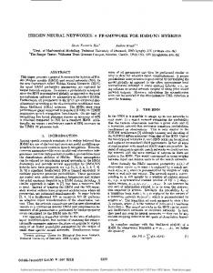
2.6 Computational expense The computational expense of the benchmark calculation is essentially proportional to the cost for matrix composition and decomposition in a single iteration and to the total number of iterations. The single-iteration composition cost is governed by the function evaluations needed to compose the element matrices of Eq. (3-4): it is hence proportional to the total number of integration points in the simulation domain, equal to the product of the number of elements in the discretisation and the number of integration points per element. The single-iteration decomposition cost on the other hand is governed by the number of equations to solve, which is directly linked to the total number of discretisation nodes in the simulation domain. It will be established that appropriately chosen numerical integration decreases the numbers of required integration points and discretisation nodes, hence reducing the matrix (de)composition costs and the total computational expense. These single-iteration costs are the main focus of this article. The use of larger elements however also has a positive influence on the time steps [7], an effect that is also observed in this analysis. This (indirect) benefit can only be appreciated. 3. DISCRETISATION AND INTEGRATION ERRORS 3.1 Illustration of integration errors To illustrate the distinction between discretisation and integration errors in non-linear finite-element simulations, and to point out the deficiency of low-order numerical integration, the benchmark calculation is executed with different spatial discretisations (A ranging from 10 to 500) and different numerical integrations (3, 7, 15 Kronrod-Patterson & 101 trapezoidal). The 101-point trapezoidal scheme is assumed to give a near-perfect integration, and simulations using that scheme should only suffer from discretisation errors. Deviations between those solutions and solutions with other integration schemes can thus be attributed to integration errors. Figure 4 presents the calculated mass absorption for the ‘500’ mesh in combination with the 101-, 15-, 7- and 3-point integration schemes. The ‘101-point’ solution is indistinguishable from the reference solution (not shown in figure), confirming hence that the ‘500’ mesh is an appropriate discretisation, and that the deviations are not caused by discretisation errors. It is clear, on the other hand, that the numerical integration has a huge impact on the results: the solutions rapidly deteriorate for lower-order integration schemes, due to integration errors. A comparison of the mass error E – Eq. (11) – for the different calculations is gathered in Figure 5. For the simulations using the reference 101-point numerical integration scheme, the error E rises monotonously with the spatial discretisation’s shape factor A: coarser spatial discretisations yield larger deviations. It should be noted though that the E for the '500’ mesh – which uses just 17 nodes – is still lower than 1 %. The effect of the discretisation errors on the benchmark calculation hence remains limited. The deviations E however quickly grow if less accurate numerical integration schemes are used. For the ‘500’ mesh, the 15-point scheme leads to E 3 %, the 7-point scheme E 44 % and the 3-point E 69 %. For all other meshes, Figure 5 also clearly indicates that the integration errors vastly overshadow the discretisation errors. To attain the 1 % accuracy with the 15-, 7- and 3-point integration schemes, one has to employ respectively the ‘250’, ‘100’ and ‘25’ meshes. This implies that reduction of the integration errors through the local concentration of discretisation nodes – be it in adaptive or immobile meshes – is effective but inefficient: it requires more discretisation nodes and integration points than really needed, unnecessarily raising the computational cost. For example, the ‘250 & 15-point’ combination requires only 25 discretisation nodes and 180 integration points (15 in each of the 12 elements), while the ’25 & 3-point’ case requires 195 discretisation nodes and 291 integration points (3 in each of the 97 elements).

6


On the whole, Figure 5 confirms that the common application of low-order numerical integration in unsaturated flow models results in substantial integration errors, which are usually far more important than the discretisation errors. While their effect can be minimised by refining the spatial discretisation, this unnecessarily increases the computational expense. An alternative approach, directly targeting the integration errors, is presented later on in this article. 3.2 Cause of integration errors The adverse effect of low-order numerical integration is obviously caused by an inaccurate numerical integration of the element matrices of Eq. (3-4). To illustrate that, a simplified version of Eq. (4) is considered here: (12) K  k m d



e

where Ωe is [-1,1], the typical domain of a one-dimensional master element. We focus on the permeability matrices here, a similar elaboration is possible for the capacity matrices. Exemplarily, the capillary pressures at the three element nodes are set -3.0·104, -3.0·105 and -1.0·106 Pa, common values for the capillary pressure fronts of the benchmark calculation. Figure 6 shows the variations of capillary pressure and moisture permeability over the element, combined with the integration points from the 3-, 7- and 15point integration schemes. It is evident that the 3-point integration scheme can not accurately integrate K: the integration points do not capture the high km region at the left side of the element, thus underestimating K. This becomes progressively better when more integration points are used. The ‘correct’ value for the integral in Eq. (12) is 1.27 ·10-10: the 15-, 7-, 3-point schemes lead to respectively 1.27·10-10, 1.20·10-10, 3.56·10-11. While the 15-point scheme gives a satisfactory result, the 7- and 3-point schemes progressively underestimate the integral. It is thus demonstrated that low-order numerical integration is not sufficient at sharp moisture fronts, and must lead to numerically erroneous simulation results. As the underestimation of permeability integrals by low-order numerical integration is limited to sharp moisture fronts, and furthermore depends on the capillary pressures involved, its occurrence is irregular. The global effect however of the irregular underestimation of the permeability matrices – and, as can be shown, also of the capacity matrices – is an underestimation of the moisture absorption, as is evident from Figure 4. 4. ADAPTIVE NUMERICAL INTEGRATION 4.1 Introduction General application of high-order numerical integration requires less computational expense than low-order integration: the ‘250 & 15-point’ and the ’25 & 3-point’ yield similar accuracy, but the latter requires 195 discretisation nodes and 291 integration points, in contrast to just 25 discretisation nodes and 180 integration points for the former. The accuracy – and computational expense – of high-order numerical integration is though only needed at the actual front: general application is neither required nor efficient. Accordingly, an adaptive numerical integration algorithm can save computation time where possible and provide accuracy where required, by adapting the density of integration points to the local non-linearity. Being originally developed to resolve non-smooth integrands, adaptive numerical integration now finds general application in the Boundary Element Method, as (near)singular integrands are typical for the boundary element matrices [17-19]. Adaptive numerical integration similarly finds its way into the eXtended Finite Element Method [20]. For the Finite Element Method on the other hand, application of adaptive numerical integration appears limited to elasto-plastic shell elements [21-22]. In [21], the numerical integration algorithm chooses between a 1- and 4-point rule, based on the state of the ele-

7


ment: 1 point for elements in the elastic regime and 4 points for elements in the plastic regime. This approach is further elaborated in [22], where the number and location of the integration points is determined from the stress distribution in the element. This article presents an iterative and a non-iterative adaptive numerical integration technique for non-linear finite-element simulations of unsaturated moisture flow in porous media, based on the nested Kronrod-Patterson 3-, 7- and 15-point rules. A first version of this technique was presented in [23]. 4.2 Iterative adaptive integration In the iterative adaptive integration, the numerical integration of the element matrices of Eq. (3-4) is progressively refined – by consecutive application of the 3-, 7- and 15-point Kronrod-Patterson rules – until convergence is reached. The computational cost of this iterative refinement is reduced by the nested Kronrod-Patterson rules: the function evaluations from the lower-level scheme can be reused by the higher-level scheme, it only requires multiplications with different weights. The capacity and permeability matrices are not considered separately however, but in their typical combination Ce + Δt·Ke from Eq. (5):

Cej1  t  K ej1  Cej  t  K ej Cej1  t  K ej1

 int egr

(13)

where j (+1) is the level of numerical integration and δintegr is the target error. Every iterative integration starts with the 3-point scheme. To evaluate the accuracy of its result, the 7-point result is calculated, and both are compared via Eq. (13). If convergence is reached, the 7-point result is maintained for the further calculation, since it is available anyway. If convergence is not reached, the 15-point result is calculated and compared to the 7-point result. If convergence is not reached at that stage, no further refinement is executed, instead the element matrices are accepted as is. Further levels could be inserted into the adaptive scheme, but given the fair performance of the 15-point scheme for our benchmark calculation (see Figure 5), this option is not pursued here. Bond [24] introduced an alternative method to assess the accuracy of a numerical integral, without the need for additional function calls. He suggests approximating the integral based on all but one of the original integration points, in combination with different weights. This approach could indeed be less costly, but chances are it is inefficient for the considered case: if the omitted integration point belongs to the region with very low km values (Figure 6), its omission would not yield a significantly different integration result. The similarity between the two integrals is however no guarantee of their accuracy. The addition of a single integration point would similarly not be efficient. The addition of multiple integration points, as proposed here with the use of the Kronrod-Patterson scheme, is on the other hand bound to give a reliable assessment. For the analysis at hand, δintegr has been taken equal to 1 %, 3 %, 5 %, 10 % and 20 %. The two larger values produce erratic deviations E from the reference solution, and are therefore not retained. The three smaller values essentially yield the same performance as the original 15-point integration in Figure 5, implying that the computational cost for matrix decomposition remains equally low. The computational cost for matrix composition however changes significantly, as the use of 15 integration points per element now becomes exceptional. For δintegr 5 %, Figure 7 shows the relative use of the 3-, 7and 15-point integration schemes for the different spatial discretisations and the average number of integration points per element. Figure 7 confirms that, for all discretisations considered, the largest share of the element integrations attain convergence at the 3-point/7-point comparison, whereas only a small share needs more integration points.

8


The average number of integration points per element consequently drops from 15 to a value between 7 and 9. While this clearly demonstrates the potential of the iterative adaptive numerical integration, there obviously also is room for improvement. As, on the one hand, the 7-point result is needed for evaluation of the 3-point result and, on the other hand, the refinement does not proceed beyond 15 integration points, the iterative adaptive numerical integration scheme essentially selects between the 7- and 15-point schemes. A non-iterative adaptive numerical integration scheme can further reduce the total number of required integration points and thus the computational cost for matrix composition. 4.3 Non-iterative adaptive integration Instead of iteratively improving the integration based on the error estimator in Eq. (13), the non-iterative scheme uses an error indicator to determine the number of integration points required for each element. The error indicator is the variation of the permeability km and capacity cm over the element, since the accuracy of the numerical integration of the element matrices in Eq. (3-4) highly depends on those. At the start of each time step, the variation of km and cm over each element is evaluated by calculating their values at the element’s nodes and determining the ratio of the maximum and minimum km and cm values. Via heuristic investigation it is concluded that the following decision algorithm leads to good results:

k max  m,max k  m,min k max  m,max k  m,min k max  m,max k  m,min

c m,max    100  15 integration points cm,min   c , m,max   5  7 integration points cm,min   c , m,max   5  3 integration points cm,min 

,

(14)

The decision on the number of required integration points is based on evaluations of km and cm at the discretisation nodes only, and is solely performed at the start of each time step: the computational expense related to this assessment is hence negligible. While it would be preferable to make this assessment at the start of each iteration, the choice for the time step level is a compromise between computational expense and efficiency. Any integration error resulting from significant shifts in the km and cm values during such time step is accepted as a consequence of this choice. This non-iterative adaptive numerical integration scheme again delivers a performance similar to that of the original 15-point scheme (Figure 5), however at a drastically lower matrix composition cost. Figure 8 shows the relative use of the 3-, 7- and 15-point integration schemes for the different spatial discretisations and the average number of integration points per element. Figure 8 confirms that the 3-point scheme suffices for most of the element integrations, lowering the average number of integration points per element to a value between 4 and 7. 4.4 Conclusion In this study, it is demonstrated that the general preference for low-order numerical integration adversely influences the needed discretisation for unsaturated moisture flow simulations. This adverse effect is attributed to the inaccurate numerical integration of the element capacity and permeability matrices, resulting from the highly non-linear relation between capillary pressure and moisture capacity and permeability. While general use of high-order numerical integration can hence be advocated, its efficiency can

9


be improved by introduction of adaptive integration, be it iterative or non-iterative. The analysis shows that an accuracy E of 1 % in the benchmark simulation requires:  general 3-point integration: 195 discretisation nodes, 291 integration points;  general 15-point integration: 25 discretisation nodes, 180 integration points;  iterative adaptive integration: 25 discretisation nodes, 101 integration points;  non-iterative adaptive integration: 25 discretisation nodes, 71 integration points; (values taken for the ‘25’ mesh for the general 3-point integration, for the ‘250’ mesh for all other integrations). For highly non-linear finite element simulations, adaptive integration can hence provide accuracy where required and efficiency where allowed. For the benchmark simulation, the use of adaptive integration – instead of the common low-order integration – allows reducing the number of required discretisation nodes with a factor 8 and the number of required integration points with a factor 4. The computational costs for matrix composition and decomposition are thus drastically decreased. As a side note, the analysis in [7] points out that larger elements also require less time steps or iterations to reach a certain temporal accuracy. This effect can be observed here as well: the number of iterations required for simulations with the ‘250’ mesh lies four times lower than the number for the ‘25’ mesh. Adaptive integration, and the consequently larger size of elements, hence also positively affects the computational cost via the total number of time step or iterations, albeit indirectly. 5. TWO-DIMENSIONAL APPLICATIONS While adaptive integration has been developed and illustrated above for a one-dimensional case, its applicability with multiple dimensions and other materials is demonstrated below. 5.1 Two-dimensional wetting of brick The first two-dimensional example concerns the capillary absorption by a square beam of ceramic brick of 0.2 x 0.2 m from a partial water contact in the centre of the material, due to a saturated 2 cm crack. Application of symmetry allows formulating the problem with these initial and boundary conditions: (15) t  0 s : x, y  [0.0;0.1] m pc  108 Pa

t  0s:

x = 0.0 m & y  [0.0;0.01] m

pc  0 Pa

other boundaries

g m  0 kg / m²s

(16)

Simulations are continued for 5000 s with alphanumeric output every 100 s. All spatial discretisations are developed based on the one-dimensional discretisations as applied in the benchmark simulation: the application of Eq. (10) in two dimensions gives the basis for meshes using quadratic 8-noded rectangular elements. Numerical integration is similarly based on a two-dimensional extension of the 3-, 7-, and 15-point Kronrod-Patterson schemes. The overall error – caused by discretisation and integration errors – is quantified with Eq. (11). Computational cost is, as before, related to the required number of discretisation nodes and integration points. For this case four different integration schemes are used: the 3-point and 15-point standard schemes and the iterative (δintegr 5 %) and non-iterative adaptive schemes. Figure 9 shows the error E for the 3-point and 15-point schemes, illustrating the importance of high-order integration again: the 15-point scheme allows reaching a 1 % accuracy with about 1500 discretisation nodes and 112.500 integration points (225 in each of the 500 elements) (values taken between the ‘100’ and ‘200’ mesh). For such accuracy, the 3point scheme needs some 30.000 nodes and 90.000 integration points (9 in each of the 10.000 elements) (values taken between the ‘20’ and ‘30’ mesh).

10


Adaptive integration schemes essentially give the same accuracy as the 15-point scheme, but with reduced matrix composition costs: the iterative and non-iterative adaptive integration need respectively about 64 and 40 integration points per element (values taken between the ‘100’ and ‘200’ mesh), instead of the original 225. As before adaptive integration gives a vast improvement over the common low-order integration, given the resulting reduction in required integration points and discretisation nodes. 5.2 Two-dimensional drying of mortar A second two-dimensional example concerns the isothermal drying of a cement mortar beam of 0.2 x 0.2 m. The beam is originally at capillary moisture content, and dries out by vapour exchange with an environment at 20 °C and 70 % relative humidity. Material properties for the cement mortar are gathered in the appendix. While actually requiring a convective boundary condition, the simulation is simplified by imposing a fixed capillary pressure of -5 107 Pa – corresponding to 70 % RH – at the drying surfaces. Application of symmetry allows formulating the problem with these initial and boundary conditions: t  0 s : x, y  [0.0;0.1] m pc  0 Pa (15)

t  0s:

pc  5 107 Pa

x or y  0.0 m

g m  0 kg /  m²  s 

x or y  0.1 m

(16)

5

Simulations are continued for 5 10 s with alphanumeric output every 104 s. The overall error – caused by discretisation and integration errors – is quantified similarly to Eq. (11), with mi now describing the total mass of lost moisture in the actual and reference solution at the output moment i. Figure 10 shows the error E for the 3-point and the 15-point schemes, once more illustrating the importance of high-order integration: the 15-point scheme reaches 1 % accuracy with 133 discretisation nodes and 8100 integration points (225 in each of 36 elements) (values taken for the ‘1000’ mesh). The 3-point integration scheme requires about 12.000 discretisation nodes and 36.000 integration points (9 in each of the 4000 elements) (values taken between the ‘30’ and ‘60’ mesh). The two adaptive integration schemes again deliver a similar performance as the 15-point scheme, but at lower matrix composition costs: the iterative and non-iterative schemes require respectively 120 and 107 integration points per element (values taken for the ‘1000’ mesh). As before, adaptive integration is a clear improvement over common low-order integration. 6. CONCLUSION Most simulation models for unsaturated moisture transfer in porous materials employ a finite-element spatial discretisation, with the element integrals generally being resolved by low-order numerical integration. This article has shown that this low-order integration is not the optimal choice for the highly non-linear unsaturated moisture transfer problem: it was demonstrated that low-order numerical integration necessitates small elements to limit the integration errors. In response to that, the efficiency of high-order integration has been illustrated: far larger elements could be used, indicating that, for highly non-linear finite-element simulations, the discretisation errors are insignificant in comparison to the integration errors. Whereas the general application of high-order integration does not yield an explosion of integration points – consequence of the ensuing reduction in number of discretisation nodes and elements –, its accuracy is actually only required at the actual moisture front, while low-order integration can be accepted in the less non-linear regions. Therefore, adaptive integration has been introduced, continuously adapting the density of integration points to the reported non-linearity.

11


Both the iterative and the non-iterative adaptive integration algorithm are based on the nested 7- and 15-point Kronrod-Patterson extensions of the common 3-point Gauss integration. In the iterative approach, the integration is progressively refined until a convergence criterion is met, while a heuristic algorithm selects the number of required integration points in the non-iterative approach. The cases considered in this paper show that the application of adaptive integration – instead of the common low-order integration – significantly reduces the number of required discretisation nodes and integration points, and thus the computational costs. While seemingly exclusive to finite-element based models, other discretisation methods – finite differences or control volumes – can equally benefit from adaptive numerical integration. Kalagasidis et al. [25] evaluated different averaging schemes for the internode permeabilities in a finite-volume-discretisation based simulation of free water uptake in ceramic brick, and observed that integral averaging performed best. A general applicability of integral averaging also requires numerical integration schemes, which hence also calls for the application of adaptive numerical integration. It should in conclusion be stated that mesh-adaptive methods outperform the adaptive numerical integration presented here. The former do necessitate far more complex implementations though, while the adaptive numerical integration technique solely needs three integration schemes. Both approaches are complementary however, and can be easily combined. APPENDIX The moisture retention curve of the considered materials is numerically described with a multimodal van Genuchten curve: n w  w cap . li . 1   ai .pc  i   

 mi

mi  1  1 ni

with

(17)

where w [kg/m3] is the moisture content, pc [Pa] is the capillary pressure, and wcap, ai, ni and li are fitting parameters. The moisture permeability km comprises the liquid permeability km,l [kg/(m·s·Pa)] and the vapour permeability km,v [kg/(m·s·Pa)], respectively described with a multimodal Durner expression and an expression taken from [15]:

k m,l  K cap   S j  with

k m,v 





 lj 1  1  S1/m j



nj S j  1   a j .pc     5 2.6110 Sap v



R2v T 2 0.503Sa 2  0.497



m 2

 

m j

(18) &

with

mj  1 1 nj Sa  1  w w cap

where pv [Pa] is the vapour pressure, Rv [kg/(J·K)] is the vapour constant for water, T [K] is the temperature, ρℓ [kg/m3] is the density of water, and Kcap, τ, aj, nj, lj and μ are fitting parameters. For reasons of flexibility, the a, n, l factors differ for the moisture retention curve and the liquid permeability description. The parameters for the ceramic brick and the cement mortar are listed in Table 3. REFERENCES [1]. Jaffer SJ, Hansson CM. The influence of cracks on chloride-induced corrosion of steel in ordinary Portland cement and high performance concretes subjected to different loading conditions. Corrosion science 2008; 50(12): 3343-3355. [2]. Pasanen A-L, Kasanen J-K, Rautiala S, Ikäheimo M, Rantamäki J, Kääriäinen H, Kalliokoski P. Fungal growth and survival in building materials under fluctuating

12


[3]. [4]. [5]. [6].

[7]. [8]. [9]. [10]. [11]. [12]. [13]. [14]. [15].

[16]. [17]. [18]. [19].

moisture and temperature conditions. International Biodeterioration & Biodegradation 2000; 46: 117-127. Fang L, Clausen G, Fanger PO. Impact of temperature and humidity on the perception of indoor air quality. Indoor Air 1998; 8(2): 80-90. Janssen H, Blocken B, Carmeliet J. Conservative modeling of the moisture and heat transfer in building components under atmospheric excitation. International Journal of Heat and Mass Transfer 2007; 50: 1128-1140. Milly PCD. Moisture and heat transport in hysteretic, inhomogeneous porous media: a matric head-based formulation and a numerical model. Water Resources Research 1982; 18: 489-498. Šimůnek J, Huang K, van Genuchten M Th. The HYDRUS code for simulating the one-dimensional movement of water, heat, and multiple solutes in variablysaturated media (Technical manual version 6.0), Research Report nr. 144, University of California Riverside, California, United States, 1996. Kavetski D, Binning P, Sloan SW. Adaptive backward Euler time stepping with truncation error control for numerical modelling of unsaturated fluid flow. International Journal for Numerical Methods in Engineering 2002; 53: 1301-1322. Thomas HR, Rees SW, Sloper NJ. Three-dimensional heat, moisture and air transfer in unsaturated soils. International Journal for Numerical Methods in Geomechanics 1998; 22: 75-95. Roels S, Carmeliet J, Hens H. Mesh adaptive finite element formulation for moisture transfer in materials with a critical moisture content. International Journal for Numerical Methods in Engineering 1999; 46: 1001-1016. Huerta A, Rodriguez-Ferran A, Diez P, Sarrate J. Adaptive finite element strategies based on error assessment, International Journal for Numerical Methods in Engineering 1999; 46: 1803-1818. Celia MA, Bouloutas ET, Zarba RL. A general mass-conservative numerical solution for the unsaturated flow equation, Water Resources Research 1990; 26: 1483-1496. Reddy JN, Gartling DK. The finite element method in heat transfer and fluid dynamics (second edition). CRC Press, Boca Raton, 2001. Huang K, Mohanty BP, Van Genuchten MTh. A new convergence criterion for the modified Picard iteration method to solve the variably saturated flow equation, Journal of Hydrology 1996; 178: 69-91. Scheffler GA. Validation of hygrothermal material modelling under consideration of the hysteresis of moisture storage. Doctoral thesis, Dresden University of Technology, Dresden, Germany, 2008. Hagentoft C-E, Kalagasidis AS, Adl-Zarrabi B, Roels S, Carmeliet C, Hens H, Grunewald J, Funk M, Becker R, Shamir D, Adan O, Brocken H, Kumaran K, Djebbar R. Assessment method of numerical prediction models for combined heat, air and moisture transfer in building components: benchmarks for onedimensional cases. Journal of Thermal Envelope and Building Science 2004; 27: 327-352. Patterson TNL. The optimum addition of points to quadrature formulae. Mathematics of Computation 1968; 22: 847-856. Li BQ, Cui X, Song SP. The Galerkin boundary element solution for thermal radiation problems. Engineering Analysis with Boundary Elements 2004; 28: 881892. Davies TG, Gao X-W. Three-dimensional elasto-plastic analysis via the boundary element method. Computers and Geotechnics 2006; 33: 145–154. Hematiyan MR. A general method for evaluation of 2D and 3D domain integrals without domain discretization and its application in BEM, Computational Mechanics 2007; 39: 509–520.

13


[20]. Benvenuti E, Tralli A, Ventura G. A regularized XFEM model for the transition from continuous to discontinuous displacements. International Journal for Numerical Methods in Engineering 2008; 74:911-944. [21]. Harn W-R, Belytschko T. Adaptive multi-point quadrature for elastic-plastic shell elements. Finite Elements in Analysis and Design 1998; 30: 253-278. [22]. Burchitz IA, Meinders T. Adaptive through-thickness integration for accurate springback prediction, International Journal for Numerical Methods in Engineering 2008; 75: 533-554. [23]. Janssen H, Carmeliet J. Adaptive integration of element matrices in finite element moisture transfer simulations. Proceedings of the XVI International Conference on Computational Methods in Water Resources, Copenhagen, Denmark, 2006. [24]. Bond C. A new integration method providing the accuracy of gauss-Legendre with error estimation capability. http://www.crbond.com/papers/gbint.pdf, 2003; accessed on May 1 2009. [25]. Kalagasidis AS, Bednar T, Hagentoft C-E. Evaluation of the interface moisture conductivity between control volumes – comparison between linear, harmonic and integral averaging. Proceedings of the International Conference on the Performance of Exterior Envelopes of Whole Buildings IX, Clearwater Beach, California, United States, 2004.

14


List of tables: 1. Overview of first internode distance, internode growth factor, number of discretisation nodes, number of elements for the different discretisations generated with A’s from 10 to 1000 2. Coordinates and weights for the standard 3-point gauss integration and the 7- and 15-point Kronrod-Patterson extensions (rounded numbers, for illustration purposes only, see [16] for more accurate presentation). 3. Fitting parameters for description of moisture retention curve and liquid and vapour permeability of ceramic brick and cement mortar.

List of figures: 1. Moisture retention curves and moisture permeability curves for ceramic brick and cement mortar. 2. Capillary pressure and moisture content profiles during water uptake by 10 cm ceramic brick, with profiles shown at 100, 500, 1200, 2500 and 5000 s. 3. Capillary pressure and normalized moisture permeability and capacity profiles during water uptake by 10 cm ceramic brick, shown at 100 s. 4. Comparison of mass absorption for the ‘500’ mesh and the 101-, 15-, 7- and 3-point numerical integration schemes. 5. Comparison of mass error E for the 101-, 15-, 7- and 3-point numerical integration schemes for the different discretisation meshes. 6. Exemplary representation of the 15-, 7- and 3-point numerical integration schemes of a permeability element matrix. 7. Relative use (in grey) of 15-, 7- and 3-point schemes, and average number of integration points per element (in black) for the iterative adaptive integration. Integrations that reach convergence at the 3-point/7-point comparison are put under the ‘3point scheme’, those that converge at the 7-point/15-point comparison are put under the ‘7-point scheme’. All other integrations are put under the ’15-point scheme’. 8. Relative use (in grey) of 15-, 7- and 3-point schemes, and average number of integration points per element (in black) for the non-iterative adaptive integration. 9. Comparison of mass error E (in grey) for the 15- and 3-point schemes for the different discretisation meshes, and average number of integration points per element (in black) for the two adaptive integration methods. 10. Comparison of mass error E (in grey) for the 15- and 3-point schemes for the different discretisation meshes, and average number of integration points per element (in black) for the two adaptive integration methods.

15


Table 1 shape factor A first internode internode growth # of nodes # of elements shape factor A first internode internode growth # of nodes # of elements shape factor A first internode internode growth # of nodes # of elements

10 1.0·10-5 1.010 465 232 70 7.0·10-5 1.070 69 34 200 2.0·10-4 1.200 29 14

20 2.0·10-5 1.020 235 117 80 8.0·10-5 1.080 61 30 250 2.5·10-4 1.250 25 12

25 2.5·10-5 1.025 195 97 90 9.0·10-5 1.090 55 27 300 3.0·10-4 1.300 21 10

30 3.0·10-5 1.030 157 78 100 1.0·10-4 1.100 49 24 400 4.0·10-4 1.400 19 9

40 4.0·10-5 1.040 119 59 120 1.2·10-4 1.120 43 21 500 5.0·10-4 1.500 17 8

50 5.0·10-5 1.050 95 47 140 1.4·10-4 1.140 37 18 700 7.0·10-4 1.700 15 7

60 6.0·10-5 1.060 81 40 160 1.6·10-4 1.160 33 16 1000 1.0·10-3 2.000 13 6

Table 2 coordinates 0.000000 ± 0.223387 ± 0.434244 ± 0.621103 ± 0.774597 ± 0.888459 ± 0.960491 ± 0.993832

3-point 0.888888

weights 7-point 0.450918 0.401397

0.555556

0.268488 0.104656

15-point 0.225510 0.219157 0.200629 0.171512 0.134415 0.092927 0.051603 0.017002

Table 3 retention curve wcap l1 a1 n1 l2 a2 n2 l3 a3 n3

ceramic brick 157 0.3000 1.25·10-5 1.650 0.7000 1.80·10-5 6.000

cement mortar 200 0.3760 2.10·10-8 2.600 0.4400 2.30·10-7 3.100 0.1840 2.90·10-6 2.000

permeabilities Kcap

τ

l1 a1 n1 l2 a2 n2 l3 a3 n3

μ

ceramic brick 1.91·10-9 -1.631 0.8910 2.96·10-5 6.620 0.0005 4.17·10-7 1.170 0.1085 1.09·10-6 2.040 30.0

cement mortar 6.98·10-11 -1.019 0.5880 3.88·10-6 3.282 0.3940 2.98·10-7 5.072 0.0180 1.43·10-8 3.465 42.8

16


moisture perm., [kg/(m·s·Pa)]

Figure 1

moisture content, [kg/m3]

200

100

0 -1E+2

-1E+5

-1E+8

ceramic brick cement mortar

1E-08

1E-13

1E-18 -1E+2

capillary pressure, [Pa]

-1E+5

-1E+8


160

-1E+4

120

-1E+5

80

-1E+6

40

-1E+7


moisture content, [kg/m3]

Figure 2

moisture content capillary pressure 0 0.00

0.02

0.04

0.06

0.08

-1E+8 0.10

coordinate, [m]

17


1E+8

-1E+4

normalised permeability normalised capacity capillary pressure

1E+6

-1E+5

1E+4

-1E+6

1E+2

-1E+7

1E+0 0.005

0.007

0.009

0.011

0.013


normalised permeability & capacity, [-]

Figure 3

-1E+8 0.015

coordinate, [m] Figure 4

absorbed mass, [kg/m²]

10

101-point scheme 15-point scheme 7-point scheme 3-point scheme

8 6 4 2 0 0

20

40

60

sqrt(time), [s0.5]

18


Figure 5

mass error E, [-]

1E+0

1E-2

1E-4

101-point scheme 15-point scheme 7-point scheme 3-point scheme

1E-6 0

100

200

300

400

500

mesh factor A, [-] Figure 6

3-point scheme 7-point scheme 15-point scheme permeability capillary pressure

1E-09

-0E+0 -2E+5

1E-10

-4E+5

1E-11

-6E+5

1E-12

-8E+5

1E-13 -1.0

-1E+6 -0.5

0.0

0.5


moisture permeability, [kg/msPa]

1E-08

1.0

local element coordinate, [-]

19


100%

15

80%

12

60%

9 3-point scheme 7-point scheme 15-point scheme integration points

40% 20%

6 3

0%

average # of integration points

relative use of scheme

Figure 7

0 0

100

200

300

400

500

mesh factor 'A', [-]

100%

15

80%

12 3-point scheme 7-point scheme 15-point scheme integration points

60% 40%

9 6

20%

3

0%

0 0

100

200

300

400


relative use of scheme

Figure 8

500


20


1E+0

225

1E-1

150

1E-2

75 3-point scheme 15-point scheme iterative adaptation non-iterative adaptation

1E-3 0

200

400

600

800


mass error E, [-]

Figure 9

0 1000


1E+0

225

1E-2

150

1E-4

75 3-point scheme 15-point scheme iterative adaptation non-iterative adaptation

1E-6 0

200

400

600

800


mass error E, [-]

Figure 10

0 1000


21

adaptive kronrod-patterson integration of non-linear finite ... - DTU Orbit

adaptive kronrod-patterson integration of non-linear finite ... - DTU Orbit

Suggest Documents

Nonlocal description of X waves in quadratic nonlinear ... - DTU Orbit

Nonlinear Analysis of a Cross-Coupled Quadrature ... - DTU Orbit

Dispersion of the second-order nonlinear susceptibility in ... - DTU Orbit

10th International Workshop on Large-Scale Integration of ... - DTU Orbit

s Single ... - DTU Orbit

YSZ Electrode - DTU Orbit

BMC Bioinformatics - DTU Orbit

Conference paper - DTU Orbit

Molecular biology - DTU Orbit

eDNA - DTU Orbit

18 point - DTU Orbit

Environmental Science - DTU Orbit

Postprint - DTU Orbit

EDISON Project - DTU Orbit

Paper title - DTU Orbit

Euronoise 2006 - DTU Orbit

FA7 - DTU Orbit

NN ... - DTU Orbit

Postprint - DTU Orbit

ultimate strength - DTU Orbit

Integrating Wind - DTU Orbit

41 Turbine ... - DTU Orbit

Nanoscale - DTU Orbit

carisma 2012 - DTU Orbit