Adaptive MIMO Channel Estimation using Sparse Variable Step-Size NLMS Algorithms Guan Gui1, Li Xu1, Lin Shan2, and Fumiyuki Adachi3 1. Department of Electronics and Information Systems, Akita Prefectural University, Akita, Japan 2. Wireless Network Research Institute, National Institute of Information and Communication Technology, Yokosuka, Japan 3. Department of Communications Engineering, Graduate School of Engineering, Tohoku University, Sendai, Japan Emails: {guiguan,xuli}@akita-pu.ac.jp,
[email protected],
[email protected]
I.
INTRODUCTION
High-rate data broadband transmission over multiple-input multiple-output (MIMO) channel is becoming one of mainstream techniques for the next generation communication systems [1], [2]. The major motivation is due to the fact that MIMO technology is a way of using multiple antennas to simultaneously transmit multiple streams of data in wireless communications [3] and hence it can bring considerable improvements such as data rate, reliability and energy efficiency. However, coherent receivers require accurate channel state information (CSI) since the received signals are distorted by multipath fading transmission. The accurate estimation of channel impulse response (CIR) is a crucial aspect and challenging issue in coherent modulation and its accuracy has a significant impact on the overall performance of the communication system. During last decades, based on the assumption of dense CIRs, linear channel estimation methods, e.g., least squares (LS), were proposed for MIMO systems. By applying these approaches, the performance of linear methods depend only on
the size of MIMO channel. Note that narrowband MIMO channel may be modeled as dense channel model because of its very short time delay spread; however, broadband MIMO channel is often modeled as sparse channel model [4]. A typical example of sparse channel is shown in Fig. 1. 0.7
No. of overall taps: 32 No. of nonzero taps: 4
0.6
0.5
Magnitude
Abstract—To estimate multiple-input multiple-output (MIMO) channels, invariable step-size normalized least mean square (ISSNLMS) algorithm was applied to adaptive channel estimation (ACE). Since the MIMO channel is often described by sparse channel model due to broadband signal transmission, such sparsity can be exploited by adaptive sparse channel estimation (ASCE) methods using sparse ISS-NLMS algorithms. It is well known that step-size is a critical parameter which controls three aspects: algorithm stability, estimation performance and computational cost. The previous approaches can exploit channel sparsity but their step-sizes are keeping invariant which unable balances well the three aspects and easily cause either estimation performance loss or instability. In this paper, we propose two stable sparse variable step-size NLMS (VSS-NLMS) algorithms to improve the accuracy of MIMO channel estimators. First, ASCE for estimating MIMO channels is formulated in MIMO systems. Second, different sparse penalties are introduced to VSS-NLMS algorithm for ASCE. In addition, difference between sparse ISSNLMS algorithms and sparse VSS-NLMS ones are explained. At last, to verify the effectiveness of the proposed algorithms for ASCE, several selected simulation results are shown to prove that the proposed sparse VSS-NLMS algorithms can achieve better estimation performance than the conventional methods via mean square error (MSE) and bit error rate (BER) metrics.
0.4
0.3
0.2
0.1
0 0
5
10
15
Tap index
20
25
30
Fig. 1. A typical example of sparse multipath channel.
Adaptive sparse channel estimation (ASCE) methods using sparse invariable step-size (ISS) least mean square algorithms (ISS-LMS) were proposed in [5]–[7] for single-input single output (SISO) channels. However, conventional ISS-LMS methods have two main drawbacks: 1) sensitive to random scale of training signal and 2) unstable in low signal-to-noise ratio (SNR) regime. To overcome the two harmful factors on channel estimation and extend their applications to estimate MIMO channels, sparse ISS normalized least mean square (ISS-NLMS) algorithms, e.g., zero-attracting ISS-NLMS (ZAISS-NLMS) and reweight ZA-ISS-NLMS (RZA-ISS-NLMS), were proposed in [8]. It is well known that step-size is a critical parameter which controls the estimation performance, convergence rate and computational cost. Different from conventional sparse ISS-NLMS algorithms [5]–[8], zeroattracting variable step size NLMS (ZA-VSS-NLMS) algorithm was proposed for ASCE to improve estimation performance in sparse multipath single-input single-output (SISO) systems [9]. Unlike the previous works, this paper proposes two sparse VSS-NLMS algorithms for estimating
sparse MIMO channels. The main contribution of this paper is summarized as follows. First, we extend the method in [9] from SISO to MIMO systems. Second, a re-weighted ZA-VSS-NLMS (RZA-VSS-NLMS) is proposed to further improve the estimation performance of MIMO channels. In addition, we explain the reason why sparse VSS-NLMS algorithms can achieve better performance than conventional sparse ISS-NLMS ones. Finally, Monte Carlo based computer simulations are conducted to confirm the effectiveness of our proposed algorithms via two metrics: bit error rate (BER) and mean square error (MSE). The remainder of this paper is organized as follows. A baseband MIMO system model is described and problem formulation is presented in Section II. In section III, sparse ISS-NLMS algorithms are reviewed and sparse VSS-NLMS algorithms are proposed. A figure example is also given to explain the difference between ISS and VSS based algorithms. Simulation results are presented in section IV in order to assess the proposed methods. Finally, we conclude the paper in Section V. Notation: Throughout the paper, capital bold letters and small bold letters denote matrices and row/column vectors, respectively; The discrete Fourier transform (DFT) matrix is denoted by F with entries [F ]kq = 1 K e − j 2π kq K , k ,q = 0, 1,..., K − 1 ; Matrices and vectors are represented by boldface upper case letters and boldface lower case letters, respectively; The superscripts (⋅)T , (⋅)H , Tr (⋅) and (⋅)−1 denote the transpose, the Hermitian transpose, the trace and the inverse operators, respectively; E (⋅) denotes the expectation operator; h 0 is the 0 norm operator that counts the number of nonzero taps in h and h p stands for the p p norm operator which is computed as h p = ( i hi )1 p , where p ∈ {1, 2} is considered in this paper; sgn(⋅) is a component-wise function which is defined by sgn(h ) = 1 for h > 0 , sgn(h ) = 0 for h = 0 , and sgn(h ) = −1 for h < 0 .
II.
z nt (t ) is an additive white Gaussian noise (AWGN) variable with distribution (0, σ n2 ) and -th received multiple-input single-output (MISO) channel vector hnr : is written as
hnr : = [hnr 1,0 , , hnr 1,L −1 , , hnr nt ,0 , , hnr nt ,L −1 hnTr 1
hnTr nt
(2)
, , hnr N t ,0 , , hnr N t ,L −1 ]T , hnTr Nt
and the matrix-vector form of system model (1) is also written as y (t ) = Hx (t ) + z (t ), (3) where received signal vector y (t ) , noise vector z (t ) and channel matrix H can be represented, respectively, as follows:
y (t ) = [y1 (t ), y2 (t ), , yNr (t )]T ,
(4)
z (t ) = [z1 (t ), z 2 (t ), , z N r (t )]T ,
(5)
T T h1T: h11 h12 T T T h22 h h H = 2: = 21 hT T T N r : hN r 1 hN r 2
h1TN t h2TN t T hN rNt
(6)
where hnr nt , nr = 1, 2, , N t , is assumed equal L -length sparse channel vector from receiver to nt -th antenna. In addition, we also assume that each channel vector hnr nt is only supported by T dominant channel taps. x
x1 x 11
…
hnr 1,0
…
x2 x 1N
x 21
xN t
…
x 2N
…
x Nt 1
…
xNtN
…
hnr 2,L −1
…
hnr N t ,0
…
hnr N t ,L −1
SYSTEM MODEL
A frequency-selective fading MIMO communication system using OFDM modulation scheme is considered. Initially, frequency domain training signal vector xnt (t ) = [x nt (t , 0),..., x nt (t , L − 1)]T , nt = 1, 2,..., N t is fed to inverse DFT (IDFT) at the -th antenna, where L is the number of subcarriers and Nt is the number of transmit antenna.2 Assume that the transmit power is normalized as E xnt = 1 . The resultant vector xnt (t ) = F H xnt (t ) is 2 padded with cyclic prefix (CP) of length LCP ≥ L to avoid inter-block interference (IBI). After CP removal, the received signal vector at the -th antenna for time t is written as ynr (t ) , where nr = 1, 2,..., N r . Then, the received signal vector y and input signal vector x (t ) are related by
ynr (t ) = n t=1 hnTr nt xnt (t ) + znr (t ) N
t
= hnTr :x (t ) + z nr
(1)
(t ),
where x (t ) = [xT1 (t ), xT2 (t ),..., xTNt (t )]T collects all of the input signal vectors from different antennas at the transmitter;
hnr 1,L −1 hnr 2,0
y nr enr (n ) Adaptive algorithm
Fig. 2. MISO channel estimation at
III.
-th antenna of the receiver.
ADAPTIVE CHANNEL ESTIMATION MEHTODS
According to the system model in Eq. (1), the n -th updating estimation error enr (n ) can be written as
enr (n ) = ynr (t ) − ynr (n ) = ynr (t ) −hnTr : (n )x (t ),
(7)
where hnr : (n ) denotes an MISO channel estimator of the hnr : (n ) ; e (n ) = [e1 (n ),e2 (n ), ,eN r (n )]T denotes receive
error vector at the receive signal at the
-th adaptive update; and ynr (t ) is the -th receive antenna.
A. Review of ZA-ISS-NLMS and RZA-ISS-NLMS For estimating hnr : (n ) as shown in Fig. 3, ZA-ISS-NLMS [7] filtering algorithm was proposed as
hnr : (n + 1) = hnr : (n ) +
μen (t )x (t ) r
T
x (t )x (t )
(
− γ ZA sgn hnr : (n )
)
(8)
where γ ZA = μλZA , λZA > 0 is a regularization parameter to balance the square estimation error enr (t ) and sparse penalty of hnr : (n ) . Motivated by reweighted ℓ -norm minimization recovery algorithm [10], Chen et al. have proposed a heuristic approach to reinforce the zero attractor which was termed as the RZA-ISS-LMS [11]. RZA-ISS-NLMS [7] was proposed as μen (t )x (t ) γ RZA sgn hnr : (n ) hnr : (n + 1) = hnr : (n ) + T r − , (9) x (t )x (t ) 1 + ε RZA hnr : (n )
(
)
where γ RZA = μλRZAε RZA , λRZA > 0 is the regularization parameter and reweighted factor ε RZA > 0 is the positive threshold. Recall that the ZA-ISS-NLMS algorithm in Eq. (8) does not make use of the VSS rather than ISS. Inspirited by the VSS-NLMS algorithm which has been proposed in [12], to improve estimation performance of MIMO channels, sparse VSS-NLMS algorithms are proposed. Unlike the sparse ISSNLMS algorithm, sparse VSS-NLMS algorithms are timevariant with respect to the accuracy of updating estimators.
Steps-size for gradient descend
1
0.8
0.6
μn (n ) = μmax ⋅ r
pTnr (n )pnr (n ) pTnr (n )pnr (n ) + C
(11)
,
where C is a positive threshold parameter which is related to received signal-to-noise ratio (SNR), C (1 SNR ) . According to Eq. (11), the range of VSS is given as μnr (n ) ∈ (0, μ max ) , where μmax is the maximal step-size of gradient descend. Theoretically, the maximal step-size is less than 2 to ensure the adaptive algorithm stability [13]. Please note that pnr (n ) in Eq. (11) is given by pnr (n ) = β pnr (n − 1) + (1 − β )
enr (n )x (t )
xT (t )x (t )
,
(12)
where β ∈ [1, 0) is a smoothing factor to trade off VSS and estimation error. C. RZA-VSS-NLMS By introducing the VSS (11) into Eq. (9), improved sparse channel estimator h (n ) is given by nr :
hnr : (n + 1) = hnr : (n ) +
(
μ (n )en (n )x (t ) γ RZA sgn hn : (n ) r
T
x (t )x (t )
−
r
1 + ε RZA hnr : (n )
) . (13)
Please note that the second term in Eq. (13) attracts the channel coefficients hn n ,l (n ) , l = 0, 1,, L − 1 whose magnitudes are comparable to 1/ǫRZA to zeros. According the two proposed filtering algorithms in Eqs. (10) and (13), adaptive channel estimation methods for estimating MIMO channels are summarized in Algorithm 1. r
t
Input: 1) x (t ) and y (t ) ; 2) μ max = 1 and C ; 3) λZA for ZA-VSS-NLMS 4) λRZA and ε RZA for RZA-VSS-NLMS. Output: channel estimator H .
Signal length: N=16 Smoothing factor: β=0.999 Threshold parameter: C=0.0001
n ← 1 ; pnr (0) ← 0 ; H (0) ← 0 ; 2 While H (n + 1) − H (n ) ≤ 10−5 or n ≥ 5000 Do 2
nr ← mod(n − 1, N r ) + 1 ; hnr : (n ) ← H (nr ;:) ;
0.4
0.2
dnr (n ) ← y (nr ); enr (n ) ← dnr (n ) −hnTr :x (n );
ISS (μ=0.5) ISS (μ=1.0) VSS (μ =0.5) max
VSS (μ
=1.0)
max
0 -5 10
10
Estimation error Fig. 3. ISS and VSS versus updating estimation error.
0
B. ZA-VSS-NLMS At time t , based on the previous research on the ZA-ISSNLMS and VSS-NLMS algorithms, ZA-VSS-NLMS algorithm is proposed as follows: hnr : (n + 1) = hnr : (n ) +
μn (n )en (n )x (t ) r
r
xT (t )x (t )
(
)
− γ ZA sgn hnr : (n ) , (10)
where μnr (n ) is the VSS which is given by
en (n )x (t ) ; pnr (n ) ← β pnr (n − 1) + (1 − β ) Tr x (t )x (t ) T pnr (n )pnr (n ) ; μnr (n ) ← μmax ⋅ T pnr (n )pnr (n ) + C μ ( n ) e ( n )x (t ) n n hnr : (n + 1) ← hnr : (n ) + r T r − γ ZA sgn hnr : (n ) x (t )x (t ) for ZA-VSS-NLMS in (10) or μ (n )enr (n )x (t ) γ RZA sgn hnr : (n ) hnr : (n + 1) ← hnr : (n ) + − xT (t )x (t ) 1 + ε RZA hnr : (n ) For RZA-VSS-NLMS in (13);
(
)
(
)
End H (nr ;:) ← hnr : (n + 1); Algorithm 1: Sparse VSS-NLMS algorithms for estimating MIMO channels.
Remark: To better understanding the difference between ISS and VSS, based on Eqs. (8) and (10), it is worth mentioning that step size μ for sparse ISS-NLMS algorithm
ISS-NLMS VSS-NLMS ZA-ISS-NLMS ZA-VSS-VNLMS RZA-ISS-NLMS RZA-VSS-VNLMS
-1
10
Average MSE
is invariable but the step size μZA (n ) for sparse VSS-NLMS algorithm is variable as depicted in as Fig. 3, where the maximal step size and ISS are set as μmax ∈ {0.5, 1.0} and μ ∈ {0.5, 1.0} , respectively. From the figure, one can easily find that ISS is kept invariant, while VSS μ (n ) decreases as the estimation performance increases and vice versa. In other words, sparse VSS-NLMS algorithms adopting VSS for adaptive gradient descend, large step-size is adopted to speed up convergence rate for reducing computational complexity; small step-size is adopted to ensure algorithm stable in the case of high-accuracy estimator for further improving estimation performance.
-2
N =N =4
10
r
t
SNR=10dB -3
10
-4
10
IV.
COMPUTER SIMULATIONS
To confirm the effectiveness of the proposed methods, two metrics, i.e., MSE and BER, are adopted for performance evaluation. Channel estimators are evaluated by average MSE which is defined by
{
2 2
},
2000
3000
4000
Iterations
and system performance is evaluated by the BER metric which adopts different data modulation schemes, such as phase shift keying (PSK) and quadrature amplitude modulation (QAM). The results are averaged over 200 independent Monte- Carlo runs. The length of each channel vector hnr nt , nr = 1, 2, , N r nt = 1, 2, , N t is set as equal length with L = 16 and corresponding number of dominant taps is set to T ∈ {1, 4} . Each dominant channel tap follows random Gaussian distribution as (0, σ h2 ) and their positions are randomly decided within the length of hnr nt . In addition, 2 MISO channel vector hnr : is subject to E hnr : = 1 . The 2 received SNR is defined as P0 σ n2 , where P0 is the power of received signal. Based on the research work in [14], it is worth mentioning that threshold parameters of sparse VSS-NLMS algorithm are adopted C = 10−4 for 5dB and C = 10−5 for 10dB and 20dB, respectively. In the first example, average MSE performance of proposed methods is evaluated in Figs. 4∼6 under two SNR regimes (i.e., 10dB and 20dB) in the case of T = 1 and 4, respectively. The effectiveness of the two proposed methods are confirmed when compared with previous methods, i.e., ISS-NLMS [13], VSS-NLMS [12] and sparse ISS-NLMS [5]–[8]. In addition, one can also find that two proposed methods depend channel sparsity as well as regularization parameter. Hence, to achieve a better steady-state estimation performance, regularization parameters for sparse VSS-NLMS algorithms, i.e., ZA-VSSNLMS and RZA-VSS-NLMS, are adopted from the paper [15], which depends on the number of nonzero taps of a channel. In addition, since sparse VSS-NLMS algorithms take advantage of the channel sparsity as for prior information, hence, they achieve better estimation performance than standard VSSNLMS algorithm, especially in a very sparse channel case, e.g., T =1.
5000
ISS-NLMS VSS-NLMS ZA-ISS-NLMS ZA-VSS-VNLMS RZA-ISS-NLMS RZA-VSS-VNLMS
(14) -1
10
Average MSE
}
1000
Fig. 4. Average MSE performance versus iterations (T = 1).
N =N =4
-2
10
r
t
SNR=10dB -3
10
-4
10
0
1000
2000
3000
4000
Iterations
5000
Fig. 5. Average MSE performance versus iterations (T = 4). ISS-NLMS VSS-NLMS ZA-ISS-NLMS ZA-VSS-VNLMS RZA-ISS-NLMS RZA-VSS-VNLMS
-1
10
-2
10
Average MSE
{
Average MSE H (n ) = E H − H (n )
0
N =N =4 t
-3
r
SNR=20dB
10
-4
10
-5
10
-6
10
-7
10
0
1000
2000
3000
Iterations
4000
Fig. 6. Average MSE performance versus iterations (T = 1).
5000
In the second example, system performance using proposed channel estimators is also evaluated with respect to BER performance. Multiple QAM schemes are considered. Received SNR is defined by Es N 0 , where Es is the average received power of symbol and N 0 is the noise power. In Fig. 7, multiple QAM schemes, i.e., 16QAM, 64QAM and 128QAM, are considered for data modulation. One can easily find that the proposed method can achieve a better estimation than previous methods.
performance than previous methods especially in high-order modulation signal based MIMO communications systems. Since the empirical parameter C is adopted for the proposed sparse VSS-NLMS algorithm in Monte Carlo runs, it may cause the performance loss in different SNR regimes. In future work, we plan to develop an adaptive C for the proposed algorithms so that it can learn the estimation error and SNR while without sacrificing much computation complexity. REFERENCES
0
10
[1]
[2]
-1
10
64QAM
128QAM
Average BER
[3] -2
10
16QAM
[4] -3
10
-4
10
-5
10
12
[5]
ISS-NLMS VSS-NLMS ZA-ISS-NLMS ZA-VSS-NLMS RZA-ISS-NLMS RZA-VSS-NLMS 14
16
18
[6] 20
22
E /N (dB) s
24
26
28
30
0
[7]
Fig. 7. Average BER performance versus received SNR (QAM). [8]
V.
CONCLUSIONS AND FUTURE WORK
Traditional adaptive MIMO channel estimation methods tend to utilize the sparse ISS-NLMS algorithms. One of the main disadvantages of the traditional methods is the inability to balance the convergence speed and the estimation accuracy on the adaptive channel estimation. In this paper, two sparse VSS-NLMS algorithms, i.e., ZA-VSS-NLMS and RZA-VSSNLMS, were proposed for estimating MIMO channels. Unlike the traditional sparse ISS-NLMS algorithms, the proposed algorithms utilized VSS which learns the estimation error and changes adaptively. Simulation results were provided to confirm the effectiveness of the proposed methods in three aspects convergence speed, estimation performance and system performance. First, convergence speed of sparse VSSNLMS based methods is faster than ISS-NLMS based methods due to the fact that VSS for adaptive gradient descend is more efficient than ISS. Second, the proposed adaptive estimators can achieve better MSE gain than traditional methods in different SNR regimes especially for sparser channels. At last, system performance using the proposed channel estimators can also achieve better BER
[9]
[10]
[11]
[12]
[13] [14]
[15]
F. Adachi and E. Kudoh, “New direction of broadband wireless technology,” Wireless Communications and Mobile Computing, vol. 7, no. 8, pp. 969–983, May 2007. D. Raychaudhuri and N. Mandayam, “Frontiers of wireless and mobile communications,” Proceedings of the IEEE, vol. 100, no. 4, pp. 824– 840, Apr. 2012. A. M. Sayeed, “Deconstructing multiantenna fading channels,” IEEE Transactions on Signal Processing, vol. 50, no. 10, pp. 2563–2579, Oct. 2002. N. Czink, X. Yin, H. OZcelik, M. Herdin, E. Bonek, and B. Fleury, “Cluster characteristics in a MIMO indoor propagation environment,” IEEE Transactions on Wireless Communications, vol. 6, no. 4, pp. 1465– 1475, Apr. 2007. O. Taheri and S.A. Vorobyov, “Sparse channel estimation with lpnorm and reweighted l1-norm penalized least mean squares,” in IEEE International Conference on Acoustics, Speech, and Signal Processing (ICASSP), Prague, Czech Republic, 22-27 May 2011, pp. 2864-2867. O. Taheri and S.A. Vorobyov, “Decimated least mean squares for frequency sparse channel estimation,” in IEEE International Conference on Acoustics, Speech, and Signal Processing (ICASSP), Kyoto, Japan, 25–30 Mar. 2012, pp. 3181–3184. G. Gui and F. Adachi, “Improved least mean square algorithm with application to adaptive sparse channel estimation, EURASIP Journal on Wireless Communications and Networking, vol. 2013, no. 1, pp. 1–18, Aug. 2013. G. Gui and F. Adachi, “Adaptive sparse channel estimation for timevariant MIMO-OFDM systems, in International Wireless Communications and Mobile Computing Conference (IWCMC), Cagliari, Italy, 1-5 July 2013, pp. 878–883. G. Gui, S. Kumagai, A. Mehbodniya, and F. Adachi, “Variable is good: Adaptive sparse channel estimation using VSS-ZA-NLMS algorithm,” in International Conference on Wireless Communications and Signal Processing (WCSP), Hangzhou, China, 24-26 Oct. 2013, pp. 1–5. E. J. Candes, M. B. Wakin, and S. P. Boyd, “Enhancing sparsity by reweighted L1 minimization,” Journal of Fourier Anaysis and Applications, vol. 14, no. 5-6, pp. 877–905, Dec. 2008. Y. Chen, Y. Gu, and A. O. Hero, “Sparse LMS for system identification,” in IEEE International Conference on Acoustics, Speech and Signal Processing (ICASSP), Taipei, Taiwan, 19-24 Apr. 2009, pp. 3125–3128. H. Shin, A. H. Sayed, and W. Song, “Variable step-size NLMS and affine projection algorithms, IEEE Signal Processing Letters, vol. 11, no. 2, pp. 132–135, Sept. 2004. B. Widrow and S. D. Stearns, Adaptive signal processing. New Jersey: Prentice Hall, 1985. H. Cho and S. W. Kim, “Variable step-size normalized LMS algorithm by approximating correlation matrix of estimation error,” Signal Processcessing, vol. 90, no. 9, pp. 2792–2799, Sept. 2010. G. Gui, A. Mehbodniya, and F. Adachi, “Least mean square/fourth algorithm for adaptive sparse channel estimation,” in IEEE International Symposium on Personal, Indoor and Mobile Radio Communications (PIMRC), London, UK, 8-11 Sep. 2013, pp. 296–300.