Mar 29, 2018 - 1Heisenberg Communications and Information Theory Group, 2Quantum ... AbstractâThe problem of wideband massive MIMO channel.
Hierarchical Sparse Channel Estimation for Massive MIMO
arXiv:1803.10994v1 [cs.IT] 29 Mar 2018
Gerhard Wunder1 , Ingo Roth2 , Axel Flinth3 , Mahdi Barzegar4 , Saeid Haghighatshoar4 , Giuseppe Caire4 , Gitta Kutyniok3 1 Heisenberg Communications and Information Theory Group, 2 Quantum Information Theory Group, FU Berlin 3 Applied Functional Analysis Group, 4 Communications and Information Theory Group, TU Berlin
Abstract—The problem of wideband massive MIMO channel estimation is considered. Targeting for low complexity algorithms as well as small training overhead, a compressive sensing (CS) approach is pursued. Unfortunately, due to the Kroneckertype sensing (measurement) matrix corresponding to this setup, application of standard CS algorithms and analysis methodology does not apply. By recognizing that the channel possesses a special structure, termed hierarchical sparsity, we propose an efficient algorithm that explicitly takes into account this property. In addition, by extending the standard CS analysis methodology to hierarchical sparse vectors, we provide a rigorous analysis of the algorithm performance in terms of estimation error as well as number of pilot subcarriers required to achieve it. Small training overhead, in turn, means higher number of supported users in a cell and potentially improved pilot decontamination. We believe, that this is the first paper that draws a rigorous connection between the hierarchical framework and Kronecker measurements. Numerical results verify the advantage of employing the proposed approach in this setting instead of standard CS algorithms.
I. I NTRODUCTION Massive MIMO, i.e. deploying large number of antennas at the base station, is a key technology for 5G [1]. Although its benefits are by now well understood and documented, the critical bottleneck for massive MIMO deployment is still the acquisition of channel state information (CSI), with designs attempting to balance the conflicting requirements of training overhead and co-pilot contamination reduction, in addition to the standard requirement of computational efficiency. This problem is even more important in massive machine type communications (MTC) where accurate CSI with low-training overhead is of critical importance [2], [3]. Towards addressing these issues, one major line of works applies compressed sensing (CS) techniques in order to account for and exploit the sparsity properties of the wireless channel. The typical approach comes in two stages: first the (spatial) covariance matrix of the received signal is estimated and, second, the dedicated user channels are estimated within the estimated spatial subspaces. This approach has been mostly applied to the narrowband signaling case, exploiting the channel sparsity in the, so called, angle domain (see [4] for an overview). Extensions of CS techniques to the wideband (OFDM) massive MIMO channel have been recently considered in [5], [6], [7]. One intuitive motivation for such an approach is that, in the wideband setting, there are more degrees of freedom available so that pilot contamination induced by co-pilots in other cells is effectively combated.
Initial work has been provided in [5], arguing that with large enough resolution in angular and time domain, controlled by the number of antennas and subcarriers, the user channels become approximately mutually orthogonal so that pilot contamination diminishes. Notably, the subspace estimates are obtained through pilot coordination over multiple slots, but not primarily through sparse channel estimation. Moreover, the claimed orthogonality is not rigorous and crucially depends on the parameter setting, let alone that bandwidth (spanned by the system subcarriers) is not a free design parameter that can be set arbitrarily large. In [6], a computationally efficient CSbased CSI acquisition approach is proposed, utilizing observations from only a limited number of subcarriers and antennas. Moreover, a fine resolution of angle and time domain together with a sparse subspace tracking algorithm is proposed. The resulting algorithm shows good performance and is exploited for pilot decontamination purposes. A similar setting is also considered in [7], where a minimimum mean squared error (MMSE) channel estimator is proposed, however, requiring prior knowledge of the channel second order statistics. Generally, a two stage approach may require excessive observations in time in order to obtain an accurate estimate of the received signal covariance matrix, which may be unacceptable, e.g., in massive MTC setting. Another major problem is that the proposed CS algorithms lack rigorous performance analysis in terms of estimation error and, equally important, number of utilized subcarriers in order to achieve it. This is mainly due to the specific Kronecker-like measurement structure of the equivalent CS problem, where, as we will show, the classical CS assumptions fail to hold, entailing convergence issues and leakage effects. However, targeting low complexity algorithms as well as small training overhead, say, in future MTC applications, it is imperative to understand such structures and to derive a tailored algorithmic framework. Contributions. We propose an efficient ”one stage” uplink massive MIMO wideband (OFDM) channel estimation taking into account only the sparsity of the wideband channel into account without any additional prior knowledge. In particular, we identify that the channel estimation problem can be posed as the identification of a vector that is hierarchically sparse, i.e., it is not only sparse but its support possesses certain structural properties. This property, together with the Kroneckerlike measurement, is taken into account for the design of an efficient CS-inspired algorithm tailored for this particular setup. In addition, by extending the standard CS analysis methodology to hierarchical sparse vectors, we provide a
rigorous analysis of the algorithm performance in terms of estimation error as well as number of pilot subcarriers required to achieve it. We believe, that this is the first paper that draws a rigorous connection between the hierarchical framework and Kronecker measurements. Preliminary simulations show that exploitation of the hierarchical sparsity property leads to improved estimation performance compared to standard CS algorithms that ignore this property. Even worse, standard algorithms may completely fail in some extreme parameter settings. Obviously, this might have some profound impact on system parameters such as pilot signal design, user capacity per cell etc. P Basic notations. kxk`q := ( i |xi |q )1/q , q > 0, is the usual notion of `q -norms, kxk := kxk`2 and kXk is the Frobenius norm of matrix X. A denotes a set of cardinality |A| and [N ] denotes {0, 1, ..., N − 1}. The elements of a vector/sequence x are denoted as (x)i (or simply xi if it clear from the context). Vector xA (matrix XA ) is the projection of elements (rows) of vector x (matrix X) onto CA . means point-wise (Hadamard) product, In is the n×n identity matrix, diag(x) is the diagonal matrix with x ∈ Cn on its diagonal. AH/T is the Hermitian/transpose of matrix A. The N × D (N × N ) DFT matrix is denoted as FN,D (FN,N = FN ) with� (FN,D )m,n := e−j2πmn/N , m ∈ [N ], n ∈ [D]. CN 0, σ 2 In denotes the multivariate complex Gaussian distribution of zero mean and covariance matrix σ 2 In . A vector x ∈ CN is called s-sparse if it consists of at most s non-zero elements. The set of non-zero elements (support) of x ∈ CN is denoted as supp(x). Organization of the paper: First, we describe our signal model and formulate the channel recovery problem. Next, we briefly present the recent framework of hierarchical sparsity, which was developed by two of the authors together with co-authors in [8]. This framework is applied to the channel estimation problem under the assumption of, so called, ongrid channel parameters, and an efficient estimation algorithm is proposed. Numerical results on the performance of the algorithm are presented, demonstrating that highly accurate channel estimation can be achieved with a very small training overhead. The more general (and practical) case of off-grid channel parameters is then considered where it is shown that the framework also applies with certain modifications that take into account basis mismatch effects. II. W IDEBAND S IGNAL M ODEL We consider an uplink massive MIMO OFDM wideband channel with single-antenna users and M � 1 antenna elements at the base station corresponding to an array manifold a (·) : [0, π) → CM , which maps angular to spatial domain. Considering a uniform linear array (ULA), the array manifold is given by a (φ) = (1, e−j2πd sin φ , . . . , e−j2πd(M −1) sin φ )T . Here, d is normalized spatial separation of the ULA, which without loss of generality (w.l.o.g.) is assumed equal to 1 in the following. As is routinely done, we perform the change of variable θ = sin(φ) ∈ [0, 1) and, with a slight abuse of notation, we write the array manifold as a function of 2πθ.
Considering a discretized approximation of the interval [0, 2π) −1 by the M points {k2π/M }M k=0 , yields the steering matrix Aθ := [a(0), a(1/M ) . . . , a((M − 1)/M )] = FM ∈ CM ×M . Further, suppose there are N � 1 OFDM subcarriers located at the (angular) frequencies ω0 , ω1 , . . . , ωN −1 , where ωk := 2πk/Ts , with Ts being the OFDM symbol duration. Assuming that the maximum delay spread of the channel for all antennas is no greater than a fraction αTs , α ≤ 1, which is the case in any reasonable OFDM design, the “delay manifold” b (·) : [0, αTs ] → CN is defined as b (τ ) := (e−jω0 τ e−jω1 τ ...e−jωN −1 τ )T , which maps the delay to the frequency domain. Considering a discretized approximation of N −1 [0, Ts ] by the N points {kTs /N }k=0 , yields the steering matrix Aτ := [b(0), b(Ts /N ), . . . , b((D − 1)Ts /N )] = FN,D ∈ CN ×D where sample number D ≤ N is the discrete delay spread1 . The channel of any user is a superposition of a small number L of impinging wavefronts (paths) characterized by their delay/angle pairs {(τp , θp )}L−1 p=0 , with τp ∈ [0, αTs ], θp ∈ [0, 1), whose values are assumed to remain constant during the considered transmission interval. The channel “spatialfrequency” transfer matrix H (t) ∈ CN ×M of an arbitrary user corresponding the OFDM symbol (slot) index t ∈ Z can be then be written as [5] H (t) =
L−1 X
ρp (t) b (τp ) aH (θp ) ,
(1)
p=0
where ρp (t) ∈ C is the time-varying gain of the p-th path at slot t. Assuming that the base station observes T consecutive (pilot) OFDM slots dedicated for channel estimation, the overall received signal equals Y (t) = diag(c(t))H(t) + Z (t) , t ∈ [T ].
(2)
The matrix Z (t) ∈ CN ×M represents noise with independent, identically distributed elements as CN (0, σ 2 ). Vector c(t) := (c (t, ω0 ) , ..., c(t, ωN −1 )) ∈ CN contains the pilot symbols transmitted over slot t. For the single-cell case considered in this paper, it is reasonable to assume that users are assigned non-overlapping sets of subcarriers to transmit their pilots on, which, w.l.o.g., are set to unity, i.e., diag(c(t)) = IN . Leveraging the sparse nature of the wideband massive MIMO channel, estimation of the channel of an arbitrary user can be achieved in principle by considering only the observations from the Oτ ≤ N pilot subcarriers the user in consideration utilizes and Oθ ≤ M antennas. Let Pτ ∈ {0, 1}Oτ ×N and Pθ ∈ {0, 1}Oθ ×M denote the corresponding sampling matrices in frequency and space dimensions, respectively. We consider a random sampling in frequency and space, i.e., the Oτ pilot subcarriers are selected uniformly from the N available subcarriers and similarly for the sampled antennas. 1 In general, a denser discretized approximation for the angle and delay domains could be employed. We leave investigation of this case for future work.
In principle, identification of the continuous-valued channel parameters {(ρp , τp , θp )}L−1 p=0 can be obtained from the low−1 dimensional sketches {Pτ Y (t)PθT }Tt=0 using the, so called, (two-dimensional) super-resolution approach (see, e.g., [9]), which is an extension of the one dimensional super-resolution approaches (see, e.g., [10], [11]). Unfortunately, the numerical resolution of the two-dimensional problem is computationally intensive, rendering this approach practical only for scenarios with Oτ and Oθ up to about 10 each. Targeting low-complexity channel estimation, we consider a discretized representation of the channel matrix, which translates the physical channel sparsity to sparsity of an appropriately defined matrix that is to be identified by the estimator. In particular, let us first assume that each delay/angle pair lies exactly on the delay/angle grid corresponding to the steering matrices Aθ and Aτ , i.e., it holds (τp , θp ) = (kp Ts /N, lp 2π/M ) for some kp ∈ [N ] and lp ∈ [M ], for all p ∈ [L]. It is easy to see that, in this case, H(t) can be written as H(t) = Aτ W (t) AH (3) θ , where W (t) :=
L−1 X p=0
ρp (t)ekp eTlp
∈C
D×M
,
(4)
with en denoting the canonical basis vector of appropriate dimension with the n-th element equal to 1. Matrix W (t) is the delay-angular representation of the channel at time t, which is a sparse matrix, with only L nonzero elements out of a total M D. Note that the set of non-zero elements (support) of W (t) is the same for each t, although W (t1 ) 6= W (t2 ), for t1 6= t2 due to the time-varying path gains. The general case, i.e. when the delay/angle pairs are off the delay/angle grid, is a bit more subtle as the discretized model leads to basis mismatch effects [12]. In particular, even though the representation of (3) is still valid, the delay-angular representation matrix now equals W (t) =
L−1 X p=0
D×M ρp (t)uτp uH , θp ∈ C
(5)
where uτp ∈ CD×1 , uθp ∈ CM ×1 are defined by the equations b(τp ) = Aτ uτp , a(θp ) = Aθ uθp , respectively, for all p ∈ [L]. In general, W (t) no longer consists of only L non-zero elements due to energy leakage over the grid points [12] (see Fig. 1). As we will see, it can however (under a regularity condition) be approximated by a matrix with a so-called hierarchical sparsity pattern, for which recovery methods have recently been developed in [8]. III. P ROBLEM S TATEMENT Considering the estimation of the channel of a single user, the problem can be formulated as the estimation of the set −1 of matrices {W (t)}Tt=0 given the low-dimensional sketches T T −1 {Pτ Y (t)Pθ }t=0 . For technical reasons,√the observed ma−1 trices {Y (t)}Tt=0 are normalized by 1/ Oτ Oθ , which, of
Fig. 1. Example of support of the delay-angular channel representation W (t) for L = 3 impinging wavefronts. Left: on grid case, Right: off-grid case.
course, occurs no information loss, and, for convenience, are vectorized, resulting in � 1 vec Pτ Y (t)PθT X (t) := √ Oτ Oθ = Ψvec (W (t)) + Φvec (Z (t)) , t ∈ [T ], (6) √ where Φ := (1/ Oτ Oθ )Pθ ⊗ Pτ ∈ {0, 1}O×M N with O := Oτ Oθ and �r � �r � 1 1 Ψ := Pθ A∗θ ⊗ Pτ Aτ ∈ CO×M D (7) Oθ Oτ is the, so called, sensing matrix [13] for the observations (measurements). By repeating this vectorization procedure over the slot dimension as well, the problem can be formulated as follows. Problem 1. Find a computationally efficient estimator of � � ¯ := vec [vec(W (0)), . . . , vec(W (T − 1))]T ∈ CM DT W given the vector consisting of multiple measurements � � ¯ := vec [vec(X(0)), . . . , vec(X(T − 1))]T ∈ COT , X
under the linear model �
¯ =Ψ ¯W ¯ + Z, ¯ X
� T where Z¯ := vec [Φvec(Z(0)), . . . , Φvec(Z(T − 1))] , ¯ := Ψ⊗IT ∈ COT ×M N T with Ψ as given in (7) and with the Ψ sampling matrices Pτ ∈ {0, 1}Oτ ×N and Pθ ∈ {0, 1}Oθ ×M generated by randomly and independently selecting Oτ and Oθ rows from the identity matrices IN and IM , respectively. We also ask for the scaling of required antennas Oθ and subcarriers Oτ for reliable (in a specific approximate sense that we will made precise later) recovery. Note that we have assumed random subsampling matrices in frequency and antenna spaces, which, in turn, imply random sets of pilot subcarriers. Even though not necessarily optimal, this random subsampling approach simplifies analysis and is actually shown to achieve good performance. A naive application of standard results from compressive sensing theory [13] suggests that recovery is guaranteed as soon as T O & LT log(T N M ). (8) However, this result only holds as long as the sensing matrix of the problem satisfies certain properties, e.g. the restricted
here, originally proposed in [8] for the estimation of general hierarchically sparse vectors from linear measurements. For the channel estimation problem, it takes the following form.
Fig. 2. Calculation of the action of the T2,2,5 -operator on a vector X ∈ C3·4·5
isometry property (RIP) [13]. As we will see, the Kroneckerlike sensing matrix of this problem might not possess such properties in general, rendering a different algorithm design and analysis methodology necessary. To this end, the appropriate mathematical framework is developed in the next section ¯. by exploiting the specific sparsity structure of W IV. A LGORITHM D ESIGN E XPLOITING S TRUCTURAL P ROPERTIES OF S PARSITY This section identifies important structural properties of the −1 channel matrices {W (t)}Tt=0 , which are taken into account for designing efficient and accurate algorithms, as well as obtaining rigorous performance guarantees. For this section, the case where the path/delay values of each path lie exactly on the sampling grid is considered, i.e., W (t), t ∈ [T ], consists of exactly L non-zero elements. The general case will be treated in the next section. A. Hierarchical Sparsity and Algorithm Design The fundamental observation towards an efficient channel estimation algorithm is that the delay/angle channel representation is not only sparse, but possesses certain structural properties as well, that fall within the notion of hierarhical sparsity. Definition 1 (Hierarchical sparsity). Let s = (s1 , . . . , s` ) ˜ ∈ be `-tuples of natural numbers and consider a vector X CN1 N2 ···Nl , with integer Ni ≥ si , i ∈ {1, 2, . . . , l}. We define ˜ inductively as follows: For the hierarchical s-sparsity of X l = 1 it is exactly the same as the standard notion of sparsity (i.e., at most s1 out of N1 elements are non-zero). For l > 1, ˜ is called s-sparse if it consists of N1 blocks out of which X at most s1 are non-zero and each of the non-zero blocks is (s2 , . . . , s` )-sparse. ¯ ∈ CM DT , It is easy to see that the unknown vector W defined in Sec. III, is a level l = 3 compound vector that is (L, L, T )-sparse. Actually, for sufficiently large M , one may also expect that no more that K (1 ≤ K ≤ L) paths have the ¯ as an (L, K, T )same angle, implying further restricting W sparse vector. ¯ should be exClearly, the hierarchically sparse structure W ploited in algorithm design and analysis as it provides signifi¯ , compared to the standard cant restrictions on the support of W ¯ simply as notion of sparsity (which would characterize W T L-sparse). Towards this end, the low-complexity, hierarchical hard thresholding pursuit (HiHTP) algorithm is considered
Algorithm 1 HiHTP ¯ sensing matrix Ψ, ¯ (L, K, T ) hierRequire: measurement X, ¯ archical sparsity for W ˆ¯ (i) = 0 1: W 2: repeat � � �� ˆ¯ (i) + Ψ ˆ ¯H X ¯ −Ψ ¯W ¯ (i) 3: A(i+1) = T(L,K,T ) W � ˆ¯ (i+1) = arg min ¯ − ΨM ¯ k MNT 4: W kX M ∈C , supp(M )⊆A(i+1)
until stopping criterion is met at i = i∗ ˆ¯ (i∗ ) Ensure: (L, K, T )-sparse matrix W 5:
The algorithm follows the philosophy of model-based compressed sensing [14]: In each iteration, it first makes a gradient descent step towards minimizing a least square objective, then projects the resulting signal onto the (L, K, T )-sparse support containing the most of its energy via application of operator T(L,K,T ) (·), and subsequently solves a least squares problem restricted to that support to find the next iterate. Utilization of the projection (or thresholding) operator T(L,K,T ) is the main differentiator of the HiHTP algorithm compared to the standard HTP algorithm [13]. In particular, ˜ ∈ CN1 N2 ···Nl and any s := for any compound vector X ˜ (s1 , s2 , . . . , sl ), Ts (X) is defined as ˜ := supp Ts (X)
arg ˜ s-sparse Z
˜ − Zk. ˜ kX
(9)
The action of this operator can be computed very efficiently. First, at the lowest level, it selects the sl largest-magnitude entries (out of a total Nl entries) for each sub-block. Then, iteratively, at level k < l, it selects the sk sub-blocks (out of a total Nk sub-blocks) whose best (sk+1 , . . . , sl )-sparse approximation are largest in l2 -norm. As an example, the iterative calculation of T2,2,5 applied on a vector X ∈ C3·4·5 is illustrated in Fig. 2. B. Performance analysis Towards characterizing the algorithm performance, the authors of [8] introduced the concept of Hierarchical RIP (HiRIP) constant. ˜ ∈ CO×N1 ···N` and Definition 2 (HiRIP). Given a matrix Ψ a vector s = (s1 , s2 , . . . , sl ), we denote by δs the smallest δ ≥ 0 such that ˜ 2 ≤ kΨXk ˜ 2 ≤ (1 + δ)kXk ˜ 2, (1 − δ)kXk
(10)
˜ ∈ C N1 ···N` . Ψ ˜ is said to have the for all s-sparse vectors X hierarchical RIP (HiRIP). Note the definition of HiRIP is less general than standard RIP: Since s-sparse vectors in particular are s1 · · · s` -sparse, s1 · · · s` -RIP implies s-HiRIP, whereas s-HiRIP does not necessary imply s1 · · · s` -RIP. However, this more restricted
notion of RIP is well justified here as it explicitly takes into account the hierarchical sparsity property of the vectors that are considered in our problem. Using the HiRIP concept, the following recovery guarantee for the HiHTP algorithm can be stated. Theorem 1. (Recovery guarantee [8]) Let 3 × (L, K, T ) := (min(3L, M ), min(3K, D), T ) and suppose that the sensing ¯ in Algorithm 1 has a HiRIP constant matrix Ψ 1 δ3×(L,K,T ) < √ . 3
(11)
ˆ ¯ (i) } of the HiHTP algoThen, the sequence of estimates {W rithm satisfies ˆ ˆ ¯ −W ¯ (i+1) k ≤ κi kW ¯ −W ¯ (0) k + τ kZk, ¯ kW
for any i ≥ 0, with
κ :=
2δ3×(L,K,T ) 2 1 − δ3×(L,K,T )
!1/2
3L, N > 3K, ¯ we need to estimate the (3L, 3K, T )-HiRIP constants for Ψ. We will use the following bound for general Kronecker-type sensing matrices [?]. ˜ := M1 ⊗M2 ⊗· · ·⊗M` , where Mk ∈ Theorem 2. Suppose Ψ COk ×Nk for all k. Further suppose that, for each k, Mk has sk -sparse RIP with constant δsk . Then, with s = (s1 , . . . , sk ), ˜ satisfies (10) with a HiRIP constant Ψ δs ≤
l Y
(1 + δsk ) − 1.
(14)
k=1
The above theorem implies that sensing matrices resulting by Kronecker products will have HiRIP, provided each of the constituent matrices has the (standard) RIP.Notably, it is important to emphasize that while HiRIP is attainable, RIP may actually not: For example, it can be shown [15] that the (standard RIP-properties of a Kronecker product M1 ⊗ · · · ⊗ M` cannot be better than the RIP -properties of the weakest matrix (with respect to the total sparsity!) Mi , since δPk sk (M1 ⊗ · · · ⊗ M` ) & max`i=1 δPk sk (Mi ). Hence, to consider the HiRIP / HiHTP framework, instead of the standard RIP framework, is inevitable to obtain recovery guarantees when using sensing matrices we consider in this publication. C. Numerical Results This section demonstrates the effectiveness of the HiHTP in obtaining highly accurate channel estimates with limited pilot overhead. In all cases, an OFDM system with N = 64 subcarriers and M = 16 antennas at the base station is considered. The “spatial-frequency” transfer matrix of the user in consideration is represented as in (3) and (4), i.e., with “on grid”
angle/delay values for each path, with L = 3. The angle/delay values of each path remain constant for the T slots considered in the estimation procedure, whereas the channel gains are independent and identically distributed (i.i.d.) over slots. For each slot, the channel gains are generated PL−1 as i.i.d. complex Gaussian variables with a total power p=0 .E(|ρp (t)|2 ) = 1. The path angles {θp }L−1 p=0 are generated independently and uniformly over the angle sampling grid, however, no two paths are allowed to have the same angle. The path delays are independent and uniformly distributed over the delay sampling grid with D = 16. For this moderate number of antennas it is reasonable to consider all of them for channel estimation purposes, i.e., Oθ = M , however, the number of (randomly) selected pilot subcarriers Oθ is a design variable. Figure 3 depicts the (average) mean squared error (MSE), 1 2 ˆ N M EkH(t) − H(t)k , of the space-frequency transfer matrix ˆ ˆ (t)AH where W ˆ (t) is the estimate obtained as H(t) := Aτ W θ estimate of the delay-angular channel representation at slot t provided by HiHTP. The MSE is depicted as a function of the training overhead Oτ /N and for various values of observed slots T . The signal-to-noise ratio (SNR) was set equal to 1/σ 2 = 0 dB. It can be seen that HiHTP offers excellent estimation accuracy for a very limited training overhead. For example, for T = 1, a training overhead of around 0.08 is sufficient to achieve a MSE that is almost one order of magnitude less than the noise level. This overhead should be compared with conventional estimation approaches which would require a pilot overhead in the order of D/N = 0.25. As expected, jointly considering T > 1 slots improves performance as the algorithm incorporates the common support of the delay-angular representation of the channel over slots. The gain of increasing T is more visible in the low training overhead regime, with T = 4 sufficient to achieve almost all of the possible gain. As a comparison, the performance of the standard HTP algorithm [13] is depicted. It can be seen that, for small training overhead, HTP performance is significant worse than HiHTP, exactly due to not taking into account the hierarchical sparsity of the channel. For sufficiently large training overhead, the performance of both algorithms are the same, implying that knowledge of the sparsity structure plays no role, exactly analogous to standard estimation theory where a priori information becomes irrelevant once sufficiently many observations are obtained. Figure 4 shows the performance of HiHTP for a training overhead Oτ /N = 0.125 as a function of SNR and for various T . As expected MSE performance improves with SNR. Utilizing more than one slots is beneficial for further improving performance in the low SNR regime. V. H IERARCHICAL S PARSITY AND H I HTP P ERFORMANCE U NDER BASIS M ISMATCH The previous section identified the structural properties of the delay/angular channel representation which were exploited in order to obtain an efficient estimation algorithm (HiHTP) and obtain performance guarantees using the concept of HiRIP. However, the analysis considered the on-grid case, i.e., with
T T T T
100
we first analyze the sparse approximation error for the vectors uτp and uθp , p ∈ [L] appearing in (5). For simplicity, the case T = 1 will be considered with the results trivially extending to the multiple measurements case. The vector uθ , for θ arbitrary, is easily seen to be equal to H (1/M )FM a(θ). As shown in [5], the i-th element of uθ equals
=1 =2 =4 =8
ˆ 2 kH − Hk
�
HTP
10−1
1 MN E
(uθ )i = HiHTP
10−2
(15)
where ξi (θ) := θ − i/M is a translation of the angle θ. In the exact same fashion and for any value of τ , it holds (uτ )i =
10−3 −2 10
sin (πM ξi (θ)) −jπ(M −1)ξi (θ) e , i ∈ [M ], M sin (πξi (θ))
100
10−1 training overhead (Oτ /N)
Fig. 3. MSE of HiHTP/HTP as a function of training overhead, for various values of T (N = 64, M = 16, D = 16, L = 3, SNR = 10 dB, Oθ = M ). 100 T =1 T =2 T =4
sin (πN ηi (τ )) −jπ(N −1)ηi (τ ) e , i ∈ [N ], N sin (πηi )
(16)
where ηi (τ ) := τ − i/N . The sparse approximation properties of uτ and uθ are identified in the following lemma. Lemma 1. For any value of θ, there exists a (2Kθ +1)-sparse vector uθ,Kθ ∈ CM , with integer Kθ ≥ 1 independent of θ and M , such that 1 kuθ,Kθ − uθ k2 . √ . Kθ Similarly, for any value of τ , there exists a (2Kτ + 1)-sparse vector uτ,Kτ ∈ CD , with integer Kτ ≥ 1 independent of τ and D, with 1 kuτ,Kτ − uτ k2 . √ . Kτ
ˆ 2 kH − Hk
�
10−1
1 MN E
10−2
Proof. The proof is omitted, and deferred to [16]. 10−3
10−4 −10
−5
0
5 SNR (dB)
10
15
20
Fig. 4. MSE of HiHTP as a function of SNR (1/σ 2 ) for various values of T (N = 64, M = 16, D = 16, L = 3, Oτ = 0.125N, Oθ = M ).
the delay/angle values lying on the grid assumed by the steering matrices Aτ and Aθ . As mentioned in Sec. II, this is not the case in general leading to basis mismatch effects. This section considers this case with the analysis split into two ¯ can be approximated parts: First, we show that the matrix W by a hierarchically sparse matrix even under basis mismatch. Then, we provide conditions in terms of number of subcarriers (Oτ ) and number of antennas (Oθ ) that should be considered in order to achieve (approximate) recovery of W for a single user. A. Sparse Approximation Analysis As has been argued in the introduction, the matrix W (t), t ∈ [T ] is not exactly sparse in general. In order to get a concrete recovery result for the application of the HiHTP algorithm for this case as well, we need to quantify how well it can be approximated as (hierarchically) sparse. In order to do this,
The error estimates derived in Lemma 1 are independent of the design parameters M and N , which means that increasing them results in an increased relative sparsity (number of nonzero to total elements) for the sparse approximations of uθ and uτ , respectively. However, increasing N requires a proportional bandwdith increase, which is not always available. On the other hand, there are no such limitation on increasing M , which can safely be assumed arbitrarily large. We now use Lemma 1 to quantify the error of approximating W (t) as having a hierarchical sparse structure. Before proceeding, we will assume the following two properties for the delay/angle pairs of the channel paths. The first property imposes a separation among distinct path angles. Condition 1 (Angular separation). For any two distinct path angles θi , θj (θi 6= θj ) in the set of delay/angle pairs, it holds |θi − θj | ≥ 2Kθ /M,
whereby | · | is meant in a wrap-around sense over the interval [0, 2π). Note that angular separations is a standard assumption in this area of research, see for instance [17], [10], [9] and can be safely assumed to hold for sufficiently large M . The second assumption essentially excludes the possibility of a channel with excessively many paths having the same angle.
Condition 2 (Limited delays-per-angle). For each distinct angle θı in the set of paths angle/delay values , there exists at most K delays τk such that (τk , θı ) is in the set of delay/angle pairs. The delays-per-angle condition is furthermore very reasonable on physical grounds: multipath components with different delays travel over different paths, hence the probability of arriving at the ULA with the same angle is very small. By the same argument one excepts that a choice K = 1 is reasonable for typical propagation conditions. We can now characterize the error of approximating W (t) (for any t) by a matrix with a hierarchically sparse structure. Proposition 1. Consider an arbitrary slot t ∈ [T ]. Under the angular separation and delays-per-angle conditions, there exists a matrix WΩ (t) ∈ CD×M whose vectorized version is (L(2Kθ + 1), K(2Kτ + 1))-sparse and satisfies kW (t) − WΩ (t)k . Kθ−1 + Kτ−1 Proof. Please see Appendix A.
L �X
ρp (ti )
p=0
Clearly, W (t), t ∈ [T ], can be well approximated by a hierarchical sparse matrix WΩ (t) by choosing Kθ and Kτ sufficiently large. This, in turn, suggests incorporation of the HiHTP algorithm, treating W (t), t ∈ [T ] as (L(2Kθ + 1), K(2Kτ + 1))-sparse. B. Error/overhead tradeoff of HiHTP algorithm We now want to identify the tradeoff between estimation accuracy and number of subcarriers and antennas that should be considered in order to achieve it. The following result provides a rigorous characterization of the HiHTP recovery guarantees, taking into account the probabilistic nature of the ¯ (t) as sampling matrices and the error of approximating W hierarchically sparse. Theorem 3. Let the number of sampled antennas and subcarriers satisfy Oθ & δ −2 L(2Kθ + 1) log4 (M ), Oτ & δ −2 K(2Kτ + 1) log4 (N ), √ respectively, for some δ < 1/ 3. Then, with a probability 3 3 larger than 1 − M − log (M ) − N − log (N ) , the sequence of ˆ ¯ (i) generated by the HiHTP algorithm (Algorithm estimates W ¯ ) as (L(2Kθ + 1), K(2Kτ + 1), T )-sparse, 1) treating vec(W will obey the error bound ˆ ˆ ¯ −W ¯ (i+1) k ≤κi kW ¯ −W ¯ (i) k + τ kZk kW
T X L X
VI. C ONCLUSION In this paper, we explored hierarchical sparse estimation framework for massive MIMO channel estimation. The framework can be used to design appropriate algorithms exploiting the sparse nature of massive MIMO channel in joint angular and delay domain. In numerical simulations we show the benefit in terms of reduced pilot overhead, particular for small overhead numbers. We also extend our analysis to the general ’off-grid’ case and derive the sufficient pilot overhead scaling for perfect recovery for large signal dimension. ACKNOWLEDGMENT AF and GK acknowledge support from the DFG (Grant KU 1446/18-1), IR and JE from the DFG (EI 519/9-1), the Templeton Foundation and the ERC (TAQ), MB from the DFG (CA 1340/1-1 and WU 598/7-1, SH and GC from the DFG (CA 1340/1-1), and GW from the DFG (WU 598/7-1 and WU 598/8-1). All DFG projects are within the German priority program on ’Compressed Sensing in Information Processing’ (COSIP). GW acknowledges also support from H2020 project ONE5G (ICT-760809) receiving funds from the European Union. The authors would like to acknowledge the contributions of their colleagues in the project, although the views expressed in this contribution are those of the author and do not necessarily represent the project. A PPENDIX A P ROOF OF P ROPOSITION 1 Let us drop the index ti . For each delay/angle pair (τp , θp ), we define ıp and p through ıp := argmini |i/QN − τp |, p := argminj |j/M − θp |, and a rectangle Ωp := [ıp − Kθ , ıp + Kθ ] × [p − Kτ , p + Kτ ] := Ip × Jp ⊆ [M ] × [QN ]. Finally define Ω through Ω=
L [
Ωp .
p=0
Due to the angular separation and delay-per angle condition, Ω is an (L(2Kθ + 1), K(2Kτ + 1))-sparse support (see Figure 5.) Now we estimate L � � X H kW (ti ) − WΩ (ti )k ≤ ρp (ti )kuτp uH − u u k. τ θp p θp p=0
For each p, we estimate
� H kuτp uH k θp − uτp (uθp ) Ω � p H ≤ kuτp uθp − uτp Jp (uθp )H k
where ρ, τ are as in Theorem 1, and C is a universal constant.
+ k(uτp )Jp (uθp )H − (uτp )Ip (uθp )Ip )H k � = kuτp − uτp Jp kkuH θp k
Proof. Please see Appendix B.
. Kθ−1 + Kτ−1 .
+ C(Kθ−1 + Kτ−1 )
ρp (ti )
i=1 p=0
+ k(uτp )Jp kk(uθp )H − (uθp )Ip )H k
Ωp
Theorem 1 implies that (t+1)
kWΩ b − WΩ b
(t)
k ≤ ρt kWΩ b − WΩ b k + τ kZk.
The claim now follows from
(r) kW − W (r) k ≤ kWΩ k + kW − WΩ b −W bk
for r = 0 and r = (t + 1) and the error bound (17). R EFERENCES
Fig. 5. The angular separation condition prevents the rectangles Ωp to intersect when they are associated to different values of θ. It does not prevent intersection for different values of τ , but this does not prevent K(Kτ + 1)sparsity in each θ-block.
We used that kuτ k = kuθ k = 1 for each τ and θ, together with Lemma 1. The claim follows. A PPENDIX B P ROOF OF T HEOREM 3 Let Ω be the (L(2Kθ + 1), K(2Kτ + 1))-sparse support set b = [0, T − 1] × Ω. defined in Proposition 1. Define the set Ω b Ω is then (T, L(2Kθ + 1), K(2Kτ + 1))-sparse, and further ¯ − W b k . (K −1 + Kτ−1 ) kW θ Ω
T X L X
ρp (ti ).
(17)
i=1 p=0
Now, we utilize that the matrices Aθ and Aτ are quadratic DFT-matrices (set D = N ). Applying Theorem 12.31 from [13, p.405] together with the assumptions on Oθ and Oτ yields that − log3 (M ) • with probability larger than 1 − M � � 1 e δ3L(2Kθ +1) √ Pθ A∗θ ≤ δ, Oθ 3
•
with probability larger than 1 − N − log (N ) � � 1 e δ3K(2Kτ +1) √ Pτ Aτ ≤ δ, Oτ
e e which in particular where δe is defined through√δ = δ(2+ δ), implies that δe ≤ δ/2 ≤ 1/(2 3), so that e δ & δ.
Hence, an estimate of the form & δ −2 implies an estimate of the form & δe−2 (with another constant), whence the theorem is applicable. Since further IT trivially obeys δT = 0, Theorem 2 implies that δ(3·L(2Kθ +1),3·(L2 (2Kτ +1),T ) (Ψ) ≤ (1 + δ)2 − 1 = δ(δ + 2) 1 ≤√ . 3
[1] M. Shafi, A. F. Molisch, P. J. Smith, T. Haustein, P. Zhu, P. D. Silva, F. Tufvesson, A. Benjebbour, and G. Wunder, “5G: A Tutorial Overview of Standards, Trials, Challenges, Deployment, and Practice,” IEEE Journal on Selected Areas in Communications, vol. 35, no. 6, pp. 1201–1221, June 2017. [2] G. Wunder, P. Jung, and M. Ramadan, “Compressive Random Access Using A Common Overloaded Control Channel,” in IEEE Global Communications Conference (Globecom’14) – Workshop on 5G & Beyond, San Diego, USA, December 2015. [Online]. Available: www.arxiv.com/1504.05318 [3] G. Wunder, I. Roth, R. Fritschek, and J. Eisert, “HiHTP: A CustomTailored Hierarchical Sparse Detector for Massive MTC,” in Proc. Asilomar Conference on Signals, Systems, and Computers (Asilomar’17), Pacific Grove, USA, November 2017. [4] S. Haghighatshoar and G. Caire, “Massive mimo channel subspace estimation from low-dimensional projections,” IEEE Transactions on Signal Processing, vol. 65, no. 2, pp. 303–318, 2017. [5] Z. Chen and C. Yang, “Pilot decontamination in wideband massive mimo systems by exploiting channel sparsity,” IEEE Transactions on Wireless Communications, vol. 15, no. 7, pp. 5087–5100, July 2016. [6] S. Haghighatshoar and G. Caire, “Massive MIMO Pilot Decontamination and Channel Interpolation via Wideband Sparse Channel Estimation,” IEEE Trans. on Wireless Communications, Januar 2017, submitted. [Online]. Available: arXivpreprintarXiv:1702.07207 [7] L. You, X. Gao, A. L. Swindlehurst, and W. Zhong, “Channel acquisition for massive mimo-ofdm with adjustable phase shift pilots,” IEEE Transactions on Signal Processing, vol. 64, no. 6, pp. 1461–1476, March 2016. [8] I. Roth, M. Kliesch, G. Wunder, and J. Eisert, “Reliable recovery of hierarchically sparse signals and application in machine-type communications,” IEEE Trans. on Signal Processing, December 2016, submitted. [Online]. Available: https://arxiv.org/abs/1612.07806v2 [9] R. Heckel, V. I. Morgenshtern, and M. Soltanolkotabi, “Superresolution radar,” CoRR, vol. abs/1411.6272, 2014. [Online]. Available: http://arxiv.org/abs/1411.6272 [10] Z. Tan, Y. C. Eldar, and A. Nehorai, “Direction of arrival estimation using co-prime arrays: A super resolution viewpoint,” IEEE Trans. Sign. Proc., vol. 62, no. 21, pp. 5565–5576, 2014. [11] M. Barzegar, G. Caire, A. Flinth, S. Haghighatshoar, G. Kutyniok, and G. Wunder, “Estimation of angles of arrival through superresolution a soft recovery approach for general antenna geometries,” arXiv, 2017. [Online]. Available: https://export.arxiv.org/pdf/1711.03996 [12] Y. Chi, L. L. Scharf, A. Pezeshki, and A. R. Calderbank, “Sensitivity to basis mismatch in compressed sensing,” IEEE Transactions on Signal Processing, vol. 59, no. 5, pp. 2182–2195, 2011. [13] S. Foucart and H. Rauhut, A mathematical introduction to Compressed Sensing. Birkh¨auser, 2013. [14] R. G. Baraniuk, V. Cevher, M. F. Duarte, and C. Hegde, “Model-based compressive sensing,” IEEE Trans. Inf. Th., vol. 56, no. 4, pp. 1982– 2001, April 2010. [15] S. Jokar and V. Mehrmann, “Sparse solutions to underdetermined kronecker product systems.” Lin. Alg. Appl., vol. 431, no. 12, pp. 2437– 2447, 2009. [16] Gerhard Wunder et al, “Hierarchical sparse channel estimation and pilot decontamination for massive mimo,” to appear on arXiv, 2018. [17] E. J. Cand`es and C. Fernandez-Granda, “Towards a mathematical theory of super-resolution,” Comm. Pur. Appl. Math., vol. 67, no. 6, pp. 906– 956, 2014.