Adaptive Multi-Robot Wide-Area Exploration and Mapping Kian Hsiang Low† , John M. Dolan†§ , and Pradeep Khosla†§ Department of Electrical and Computer Engineering† , Robotics Institute§ Carnegie Mellon University 5000 Forbes Avenue Pittsburgh PA 15213 USA
{bryanlow, jmd}@cs.cmu.edu,
[email protected]
ABSTRACT The exploration problem is a central issue in mobile robotics. A complete terrain coverage is not practical if the environment is large with only a few small hotspots. This paper presents an adaptive multi-robot exploration strategy that is novel in performing both wide-area coverage and hotspot sampling using non-myopic path planning. As a result, the environmental phenomena can be accurately mapped. It is based on a dynamic programming formulation, which we call the Multi-robot Adaptive Sampling Problem (MASP). A key feature of MASP is in covering the entire adaptivity spectrum, thus allowing strategies of varying adaptivity to be formed and theoretically analyzed in their performance; a more adaptive strategy improves mapping accuracy. We apply MASP to sampling the Gaussian and logGaussian processes, and analyze if the resulting strategies are adaptive and maximize wide-area coverage and hotspot sampling. Solving MASP is non-trivial as it comprises continuous state components. So, it is reformulated for convex analysis, which allows discrete-state monotone-bounding approximation to be developed. We provide a theoretical guarantee on the policy quality of the approximate MASP (aMASP) for using in MASP. Although aMASP can be solved exactly, its state size grows exponentially with the number of stages. To alleviate this computational difficulty, anytime algorithms are proposed based on aMASP, one of which can guarantee its policy quality for MASP in real time.
myopic path planning
1. INTRODUCTION
The problem of exploring an unknown environment is a central issue in mobile robotics. Typically, it requires sampling the entire terrain. However, a complete terrain coverage is not practical in terms of resource costs if the environment is large with only a few small, dynamic “hotspots”, and the robot sensing range is limited. Such an environment arises in two important real-world applications: (a) planetary exploration such as geologic reconnaissance and mineral prospecting [9], and (b) environment and ecological monitoring such as monitoring of ocean phenomena (e.g., algal bloom) [7], forest ecosystems [13], pollution, and contamination. In these applications, it is often necessary to sample the hotspots for detailed analysis and extraction. At the same time, the environment has to be adequately covered to locate these hotspots as well as map the phenomena accurately. To reduce human effort and risk, it is desirable to build robot teams that can perform these tasks. An important issue in designing such a robot team is the exploration strategy: how do the robots decide where to explore next? This paper presents an adaptive model-based exploration strategy that is novel in performing both widearea coverage and hotspot sampling, and covering the entire adaptivity spectrum. In contrast, all other model-based strategies are non-adaptive and achieve only wide-area coverage. Our strategy can also plan non-myopic multi-robot paths, which are more desirable than greedy or single-robot Categories and Subject Descriptors paths. These characteristics distinguish our approach from G.1.6 [Optimization]: convex programming; G.3 [Probability the existing robot exploration strategies and are discussed and Statistics]: stochastic processes; I.2.8 [Problem Solvin greater detail with the related work below: ing, Control Methods, and Search]: dynamic programWide-Area Coverage vs. Hotspot Sampling Exploming; I.2.9 [Robotics]: autonomous vehicles ration strategies [7, 12, 13, 16, 17, 18] that emphasize widearea coverage aim to improve the mapping accuracy of the General Terms environmental phenomena. On the other hand, strategies that focus on locating and sampling hotspots [9] may not be Algorithms, Performance, Design, Experimentation, Theory tailored to satisfy this objective. In contrast, our proposed approach can tackle both tasks simultaneously. Keywords Model- vs. Design-Based Strategies In design-based multi-robot exploration and mapping, adaptive sampling, strategies [9, 13, 18], the selection of sampling locations for active learning, Gaussian process, log-Gaussian process, nonexploration is constrained by the sampling design, which is not devised to consider resource costs. As a result, the locaCite as: Adaptive Multi-Robot Wide-Area Exploration and Mapping, Kian Hsiang Low, John M. Dolan, and Pradeep Khosla, Proc. of 7th tions have to be chosen by the strategy first before minimizInt. Conf. on Autonomous Agents and Multiagent Systems ing the resource costs to sample them. This entails “sunk” (AAMAS 2008), Padgham, Parkes, Müller and Parsons (eds.), May, 12costs in motion; the exploration paths have to traverse ter16., 2008, Estoril, Portugal, pp. 23-30. rain that do not require sampling to reach the selected loc 2008, International Foundation for Autonomous Agents and Copyright cations. Furthermore, some strategies [13, 18] require mulMultiagent Systems (www.ifaamas.org). All rights reserved.
tiple “passes” through the region of interest such that new locations are adaptively selected and sampled in each pass. Modifying the strategy to involve resource costs may invalidate the estimators associated with the strategy. We instead use a model-based strategy [7, 12, 16, 17], which assumes a certain environmental model and selects sampling locations to reduce its uncertainty. Resource cost minimization or constraints may be applied to the selection process and the resulting strategy is optimal in these constraints. In contrast to the strategies [7, 12, 16] that use a parametric model, our approach utilizes a non-parametric model, which does not require any assumptions on the distribution underlying the sampling data. In particular, we model the environmental phenomena as Gaussian [17] and log-Gaussian processes. Adaptive vs. Non-Adaptive Sampling Strategies Adaptive sampling refers to strategies [9, 13, 18] in which the procedure for selecting locations to be included in robot paths depends on the sampling data observed during exploration. On the other hand, non-adaptive sampling strategies [7, 12, 16, 17] have no such dependence. When the environmental phenomena are smoothly varying, non-adaptive strategies are known to perform well [18]. However, if the environment contains hotspots, adaptive sampling can exploit the clustering phenomena to map the environmental field more accurately than non-adaptive sampling. In contrast to the above schemes, the adaptivity of our proposed strategy can be varied (Section 2.3); by increasing adaptivity, its mapping accuracy can be improved. Greedy vs. Non-Myopic Path Planning Strategies In contrast to greedy strategies [12, 17] that face the local minima problem, our strategy generates non-myopic robot paths [16]. Non-myopic paths usually approximate the optimal trajectories better, but incur higher computational cost. Single- vs. Multi-Robot Strategies In contrast to singlerobot exploration strategies [12, 13, 16], our strategy has to coordinate the exploration of multiple robots like those in [7, 9, 17, 18]. A robot team can potentially complete the task faster than a single robot and is also robust to failures by providing redundancy.
2.
MULTI-ROBOT ADAPTIVE SAMPLING PROBLEM (MASP)
2.1 Terminology and Notation Let X be the domain of the environmental phenomena corresponding to a finite, discretized set of grid cell locations (i.e., cell centers). Let Zx be a random variable representing the unobserved quantity at an arbitrary location x ∈ X ; its realized observed/sampled quantity will be denoted by zx . Let the data of m sampled locations d0 be an ordered list of pairs hxi , zxi i for i = 1, . . . , m. So, the addition of the data of n new sampled locations to d0 results in dn = [hx1 , zx1 i, . . . , hxm+n , zxm+n i]. Let xdn and zdn denote vectors comprising the x and zx components of the data dn respectively (i.e., xdn = (x1 , . . . , xm+n ) and zdn = (zx1 , . . . , zxm+n )). A robot path P corresponds to a sequence of l locations. When a robot travels between two locations x and y, it incurs a motion cost of C(x, y). The cost C(P) of a robot path P = hx1 , . . . , xl i is defined as the sum P of the motion costs along the path, i.e., li=2 C(xi−1 , xi ).
We will define more clearly the notion of adaptivity in an exploration strategy, which is crucial to understanding MASP. Suppose that the data d0 has been sampled previously and n new locations are to be selected for sampling. Formally, an exploration strategy is strictly adaptive if its procedure to select each new sampling location xm+i+1 for i = 0, . . . , n − 1 depends only on the previously sampled data di . A strategy is non-adaptive [7, 12, 16, 17] if its procedure to select each new sampling location xm+i+1 for i = 0, . . . , n − 1 is independent of zxm+1 , . . . , zxm+n . Hence, all the n new locations can be selected prior to exploration without needing to observe any new sampling data. By hybridizing the two, a partially adaptive [9, 13, 18] strategy results, that is, its procedure to select each batch of j new locations xm+ij+1 , . . . , xm+ij+j for i = 0, . . . , n/j − 1 1 depends only on the previously sampled data dij . When j = 1 (n), this strategy becomes strictly adaptive (non-adaptive). So, by increasing the number of new locations in each batch, the adaptivity of the hybrid strategy decreases.
2.2 Problem Formulation The exploration objective is to collect the “best” sampling data from the planned robot paths that maximizes the mapping accuracy of the environmental field. To achieve this, we use the mean-squared error criterion as a measure of the spatial mapping uncertainty. Given the previously ˆ 0 , d0 ) of the unobserved sampled data d0 , a predictor Z(x quantity Zx0 at location x0 achieves the mean-squared error ˆ 0 , d0 )]2 |d0 }. Then, the uncertainty in mapping E{[Zx0 − Z(x ˆ 0 , d0 ) the environmental field of domain X with predictor Z(x can be represented by P the sum of mean-squared errors over ˆ 0 , d0 )]2 |d0 }). Usall locations in X (i.e., x0 ∈X E{[Zx0 − Z(x ˆ 0 , d0 ) def ing the best unbiased predictor Z(x = E[Zx0 |d0 ] (i.e., it achieves the lowest mean-squared error among all unbiased predictors), the mean-squared error at each location def
2 x0 can be reduced to the conditional variance σZ = x0 |d0 |d ]. This results in the spatial mapping uncertainty var[Z 0 x 0 P 2 x0 ∈X σZx0 |d0 , which will be used in formulating the exploration problems below. In essence, the multi-robot exploration problem involves selecting new sampling locations for the robot exploration paths that provide the least amount of spatial mapping uncertainty. One typical way of doing this would be by choosing all the new locations to be added to the existing sample (say, d0 ) that minimize the expectation of the sum of posterior variances over all locations in X : X 2 min E{ (1) σZx0 |d0 ,DP1 ,...,DP | d0 } P1 ,...,Pk
k
x0 ∈X
subject to the motion constraint C(Pi ) ≤ B for robot i = 1, . . . , k where DPi is an ordered list of pairs hx, Zx i constructed from the path Pi . To interpret (1), the selection of new locations xDP1 ,...,DPk to be included in the robot paths P1 , . . . , Pk does not depend on the previously sampled data along the paths. Hence, this problem formulation is non-adaptive. On the other hand, the new locations can also be selected sequentially such that the selection of subsequent locations to be included in the robot paths depends on the previously sampled data along the paths. This form of exploration 1
to simplify exposition, we assume that n is divisible by j.
can be achieved by modeling MASP using Dynamic Programming (DP) with the following value functions, which represent the amount of spatial mapping uncertainty: Vi (dki ) =
min
ai ∈A(x k ) d
k E[Vi+1 (dki , Di+1 ) | dki ]
i
X
Vn (dkn ) =
(2)
2 σZ x0 |dkn
x0 ∈X
for i = 0, . . . , n − 1 where the realized data dki is an ordered list of the last k pairs of dki , xdk = (xm+k(i−1)+1 , . . . , xm+ki ) i is a vector of k robot locations denoting the current state of the robot team, A(xdk ) is the action space of the robot team i (i.e., a finite set of joint actions) given its current state xdk , i
k the unobserved data Di+1 is an ordered list of pairs hxℓ , Zxℓ i for ℓ = m + ki + 1, . . . , m + ki + k, and xD k is the next i+1 state produced by the deterministic transition function of the robot team T (ai , xdk ) based on its current action ai i and state xdk . To interpret (2), the selection of subsequent i locations xD k to be included in the robot paths P1 , . . . , Pk i+1 depends on the previously sampled data dki along the paths, which makes this problem formulation adaptive. Hence, the random data D1k , . . . , Dnk corresponds to the sample that is to be realized by the robot paths P1 , . . . , Pk . The above motion constraints on the robots also apply in this problem. Let π = hπ0 (d0 ), . . . , πn−1 (dk(n−1) )i denote the action def
policy of the robot team such that πi (dki ) = ai ∈ A(xdk ). i By solving (2), the optimal value V0 (d0 ) can be obtained together with the corresponding optimal action policy π ∗ where k ) | dki ] . πi∗ (dki ) = arg min E[Vi+1 (dki , Di+1
(3)
ai ∈A(x k ) d i
From (3), the optimal action π0∗ (d0 ) can be determined prior to exploration since data d0 is known. However, each action rule πi∗ (dki ), i = 1, . . . , n−1 defines the actions to take in response to the data dki , part of which (i.e., [hxm+1 , zxm+1 i, . . . , hxm+ki , zxm+ki i]) will only be observed during exploration. Given the starting locations (say, xdk ) of the robots, their 0 paths P1 , . . . , Pk can also be derived by applying the transition function T (., .) to the optimal action policy π ∗ . In some exploration tasks, a tradeoff may ensue between adaptivity and task execution cost: for example, the primary environmental variable to be mapped is sometimes associated with highly correlated auxiliary variables, which may be cheaper to sample at a higher spatial resolution or more reliable for planning the exploration paths. So, if an auxiliary variable is used in MASP for path planning instead, an adaptive strategy has to incur the extra cost of sampling the auxiliary variable during exploration, which is not required by non-adaptive exploration.
2.3 Advantage of Adaptive Exploration Increasing adaptivity can improve mapping accuracy (i.e., lower spatial mapping uncertainty) as shown below: Theorem 2.1. Define the value functions of j-MASP as Vij (dkij ) =
j k k min E[Vi+1 (dkij , Dij+1 , . . . , Dij+j ) | dkij ] aij ,...,aij+j−1 X 2 j σZ Vn/j (dkn ) = x0 |dkn x0 ∈X
(4)
for i = 0, . . . , n/j − 1 where j is the number of robot team actions per stage, xD k := T (aij+l−1 , xD k ) for l = ij+l
ij+l−1
k 1, . . . , j such that Dij := dkij , and assume n is divisible by j. j Then, V0 (d0 ) is monotonically increasing in j.
To elaborate, each stage of j-MASP in (4) consists of a minimum followed by an expectation. As the number j of robot team actions per stage decreases, the number of locations sampled per stage decreases, which implies an increase in adaptivity (Section 2.1). At the same time, the optimal value (i.e., spatial mapping uncertainty) decreases with increasing adaptivity. Note that 1-MASP corresponds to MASP in (2) while n-MASP is of the same form as the non-adaptive exploration problem in (1). The computational efficiency of j-MASP does not improve with decreasing adaptivity (i.e., increasing j): for a fixed number of new locations (i.e., kn) to be sampled, the required number of stages decreases with decreasing adaptivity. But, it is associated with increasing dimensionality of the action space under each minimum and also, of the probability distribution for each expectation. If these expectations have to be evaluated numerically, the number of value function evaluations required for each expectation has to grow exponentially with the number of locations sampled per stage for the numerical approximation to be effective. Since the action space under each minimum also grows exponentially with the number of robot team actions per stage, there is no computational gain by decreasing the adaptivity.
2.4 Alternative Formulation In this subsection, we provide an alternative formulation to MASP in (2) that lends itself to a different interpretation. More importantly, this reformulation can be subject to convex analysis (Section 2.6), which allows monotone-bounding approximation of MASP to be developed (Section 3.1). The reformulated MASP comprises the value functions Ui (dki ) =
max
ai ∈A(x k ) d
k ) | dki ] R(xD k , dki ) + E[Ui+1 (dki , Di+1 i+1
i
Ut (dkt ) =
max
at ∈A(x k ) d
R(xD k , dkt ) t+1
t
(5) for i = 0, . . . , t − 1 with t = n − 1 and the reward functions X R(xD k , dki ) = var[µZx |dki ,D k | dki ] (6) 0
i+1
i+1
x0 ∈X
def
k ]. An analog to Thewhere µZx |dki ,D k = E[Zx0 |dki , Di+1 0 i+1 orem 2.1 can be derived for the reformulated MASP except that the optimal value increases, rather than decreases, with increasing adaptivity.
Theorem 2.2. The value functions of MASPs in (2) and (5) are related by X 2 (7) σZx0 |dki − Ui (dki ) Vi (dki ) = x0 ∈X
for i = 0, . . . , n − 1 and their respective optimal action policies coincide. Theorem 2.2 can be generalized to cater to j-MASPs. The reformulated MASP in (5) is interpreted differently from the original MASP in (2): from the well-known variance decomposition formula 2 2 = E[σZ σZ x0 |dki x
k 0 |dki ,Di+1
| dki ] + var[µZx
k 0 |dki ,Di+1
| dki ],
def
|dki ] term measures the reduction in un-
µYx = E[Yx ] = exp{µZx + σZx Zx /2} and covariance func-
2 to certainty at location x0 from the prior variance σZ x0 |dki 2 the expected posterior variance E[σZx |d ,D k |dki ] by sam-
tion σYx Yy = cov[Yx , Yy ] = µYx µYy (exp{σZx Zy } − 1) for x, y ∈ X . From Section 2.5, we know that the distribution of Zx0 given dkn is Gaussian. Since the transformation from zdkn to ydkn is invertible, the distribution of Yx0 given dkn is log-Gaussian with the conditional mean and variance:
the var[µZx
k 0 |dki ,Di+1
0
ki
i+1
pling the new locations xD k . So, by exploring new locai+1 tions xD k at every stage that achieve greater reduction i+1 in uncertainty over all locations in X (i.e., maximizing rewards in (5)), we remove the largest possible amount of uncertainty from the initial spatial mapping uncertainty (i.e., P 2 x0 ∈X σZx0 |dki in (7)). This is in contrast to the original MASP in (2) whereby the cost to be minimized appears only in the last stage (i.e., final spatial mapping uncertainty P 2 x0 ∈X σZx0 |dkn ). In the next two subsections, we will show how the reformulated MASP in (5) can be applied to the Gaussian and log-Gaussian processes. In particular, we will analyze whether MASP is adaptive for these processes and the convex properties of MASP for the log-Gaussian process.
def
2 /2} µYx0 |dkn = exp{µZx0 |dkn + σZ x0 |dkn
(11)
2 } − 1) σY2 x0 |dkn = µ2Yx0 |dkn (exp{σZ x0 |dkn
(12)
2 are determined using (8) and where µZx0 |dkn and σZ x0 |dkn (9) respectively. For ℓGP, MASP is adaptive. This is a direct consequence of the following lemma:
Lemma 2.5. R(xD k , dki ) in (6) depends on dki for i = i+1 0, . . . , t.
2.5 MASP for Gaussian Process (GP)
The next theorem follows from Lemma 2.5 and (5):
Let {Zx }x∈X denote a GP defined on the domain X , that is, the joint distribution over any finite subset of {Zx }x∈X is Gaussian. The GP can be completely specified by its mean def def function µZx = E[Zx ] and covariance function σZx Zy = cov[Zx , Zy ] for x, y ∈ X . In this paper, it is assumed that the mean function and covariance structure of Zx are known. Given the previously sampled data dkn , the distribution of Zx0 is a Gaussian with the conditional mean and variance
Theorem 2.6. Ui (dki ) and πi∗ (dki ) depend on dki for i = 0, . . . , t.
µZx0 |dkn = µZx0 + Σx0 xdkn Σ−1 xd
kn
xd
kn
2 = σZx0 Zx0 − Σx0 xdkn Σ−1 σZ xd x0 |dkn
{z⊤ dkn − µZdkn } (8)
kn
xd
kn
Σxdkn x0
(9)
where µZdkn is a column vector with mean components µZxi for i = 1, . . . , m + kn, Σx0 xdkn is a covariance vector with components σZx0 Zxi for i = 1, . . . , m + kn, Σxdkn x0 is the transpose of Σx0 xdkn , and Σxdkn xdkn is a covariance matrix with components σZxi Zxj for i, j = 1, . . . , m + kn. For GP, MASP can be reduced to be non-adaptive. This is a direct consequence of the following lemma: Lemma 2.3. R(xD k , dki ) in (6) is independent of zdkt i+1 for i = 0, . . . , t. The next theorem follows from Lemma 2.3 and (5): Theorem 2.4. Ui (dki ) and πi∗ (dki ) are independent of zdkt for i = 0, . . . , t. Hence, the selection of new sampling locations xD k is ini+1 dependent of zdkt for i = 0, . . . , t. As a result, MASP for GP can be reduced to a deterministic planning problem U0 (d0 ) = max
a0 ,...,at
t X
R(xD k , dki ) , i+1
(10)
i=0
which aims to provide sufficient coverage for mapping the environmental field accurately. However, it does not account for maximization of sampling at hotspots (Lemma 2.3).
2.6 MASP for log-Gaussian Process (ℓGP) Let {Yx }x∈X denote a ℓGP defined on the domain X . That is, if we let Zx = log Yx , then {Zx }x∈X is a GP (Section 2.5). So, Yx = exp{Zx } and ℓGP has the mean function
Hence, the selection of new sampling locations xD k dei+1 pends on the previously sampled data dki for i = 0, . . . , t. Besides providing coverage to learn an accurate spatial mapping, MASP in (5) for ℓGP also maximizes hotspot sampling: it can be shown that a large reward var[µYx |dki ,D k |dki ] 0 i+1 in (6) is associated with a high expected quantity µYx0 |dki . So, if x0 is one of the new sampling locations in xD k , i+1 MASP in (5) tends to select location x0 with a large reward var[µYx |dki ,D k |dki ]. Consequently, x0 has a high expected 0 i+1 quantity, thus maximizing sampling of hotspots (i.e., areas of high measured quantities). The value functions of MASP in (5) may not be convex in the sampled quantities yd of the input data d. However, MASP can be transformed to be convex by a change of variables Zx = log Yx , x ∈ X as shown below: Lemma 2.7. R(xD k , dki ) in (6) is convex in zdki (i.e., i+1 (log yx1 , . . . , log yxm+ki )) for i = 0, . . . , t. The next theorem follows from Lemma 2.7 and (5): Theorem 2.8. Ui (dki ) is convex in zdki (i.e., (log yx1 , . . . , log yxm+ki )) for i = 0, . . . , t.
3. VALUE-FUNCTION APPROXIMATIONS The solution technique presented in this section focuses on tackling the strictly adaptive MASP in (5) (Section 2.1), which implies only one new location should be selected at each stage. The value functions can then be simplified in the following two ways resulting in (13): (a) rather than choose a joint action ai ∈ A(.) to move all robots simultaneously in each stage, only one robot should be chosen at each stage to sample a new location while the rest of the robots stay put. This tradeoff between simultaneous actions and strict adaptivity results in a reduced set A′ (.) of joint actions for the robot team that grows linearly, rather than exponentially (Section 2.3), with the number of robots; (b) consequently, k the unobserved data Di+1 can be reduced to a single pair ′ hx , Zx′ i corresponding to the new location x′ to be sampled
by the chosen robot. Since the other unselected robots are k stationary in that stage, the remaining pairs in Di+1 correspond to locations selected in the previous stages and can be found in the known data di . The probability distribution for the conditional expectation in MASP can therefore be simplified to a uni-variate Zx′ , which reduces the computational burden of solving the problem numerically (Section 2.3). Ui (di ) = Ut (dt ) =
max
R(x′ , di ) + E[Ui+1 (di , hx′ , Zx′ i)|di ]
max
R(x′ , dt )
ai ∈A′ (xi ) at ∈A′ (xt )
(13) for i = 0, . . . , t − 1 where xi is a vector of the k robot locations denoting the current state of the robot team that can be derived from the sampled locations xdi , and xi+1 is the next state produced by the deterministic transition function T (ai , xi ). Note that x′ is the component in xi+1 with the same index as the non-zero component in xi+1 − xi . Since the random variable Zx′ is continuous, an exact solution to the above MASP will not be computationally feasible if the conditional expectation is evaluated by computing Ui+1 (di , hx′ , Zx′ i) infinitely often over the support of Zx′ . For MASP with t = 1 in (13), it can be shown that the conditional expectation can be evaluated in closed form, which makes the problem computationally feasible. At this moment, we are not aware of any computationally feasible methods to solve MASP with t > 1 exactly. Hence, we will resort to approximating MASP as described below. For ease of exposition, we will revert to using the Zx variable for ℓGP (i.e., by transforming Zx = log Yx ) in the rest of this paper. The difficulty in solving the multi-stage MASP lies in evaluating the conditional expectation with respect to the continuous state variable Zx′ . This intricate issue of handling continuous states is faced by the following related stochastic decision-theoretic planning problems, which have resolved it by constructing approximate problems: Markov decision processes (MDPs) The traditional approach of generalizing to continuous states in an MDP is to approximate the value function with a parameterized model; the resulting solution is usually hard to analyze and may diverge. To make the problem computationally feasible to solve, recent approaches such as the time-dependent [8] and factored MDPs [6] approximate it by constraining the transition, reward, and value functions to certain function families. However, time-dependent MDPs suffer from an exponential blow-up with an increasing number of stages while factored MDPs induce infinitely many constraints in their linear programming formulation. In contrast, MASP adopts a more complex but realistic non-Markov structure; the transition function is conditioned on the entire history of actions and continuous states. More importantly, by assuming the reward and value functions to be convex (Section 2.6), piecewise-linear functions can be constructed to monotonically bound and approximate the value function (Section 3.1). Note that the form of the transition function is not restricted. Non-Markov problems Bayes sequential design problems [11] and stochastic programs [4, 15] can be modeled as nonMarkov DP problems. In contrast to MASP, they have a simple structure: (a) their transition functions do not depend on past actions, (b) for Bayes sequential design, the entire history of continuous states can be reduced to a summary statistic, and (c) for stochastic programs, the reward
function is often assumed to be linear in the action variable [4]. To make them computationally feasible to solve, the conditional expectation is approximated using Monte-Carlo sampling for both problems [11, 15] and bounding methods [4] for stochastic programs. The latter technique further assumes the value function to be linear or convex in the continuous state and action variables. The resulting approximate problems suffer from an exponential blow-up. Our bounding approximation technique (Section 3.1) utilizes the results on generalized Jensen bounds for convex functions [5] from the field of stochastic programming.
3.1 Approximate MASP In this section, we will formulate the approximate MASP (aMASP) whose optimal value lower-bounds that of MASP in (13). To obtain aMASP and its corresponding bound, the following result is required, which utilizes Jensen’s inequality to lower-bound the expectation of a convex function: Theorem 3.1 ([5]). Let W (ξ) be a convex function of ξ with the support [a, b] that is subdivided at arbitrary points b0 , . . . , bν (i.e., a := b0 < b1 < . . . < bν =: b). Let the ν-fold generalized Jensen bound be denoted by def
Jν =
ν X
αj W (βj ),
ν = 1, 2, . . . ,
(14)
j=1
where def
αj =
Z
bj
def
f (ξ)dξ, βj =
bj−1
1 αj
Z
bj
ξf (ξ)dξ, j = 1, . . . , ν . bj−1
If the partition corresponding to k + 1 is at least as fine as that corresponding to k for k = 1, . . . , ν −1, J1 ≤ . . . ≤ Jν ≤ E[W (ξ)]. Let the support of Zx′ given the sampled data di be Sxν′ i = [a, b] that is partitioned into ν non-empty, disjoint intervals Sxν′ ij = [bj−1 , bj ] for j = 1, . . . , ν. Using Theorem 3.1, aMASP can be derived from (13) with the structure: U νi (di ) = U νt (dt ) =
max ′
R(x′ , di ) +
max
R(x′ , dt )
ai ∈A (xi ) at ∈A′ (xt )
ν X
px′ ij U νi+1 (di , hx′ , zx′ ij i)
j=1
(15) def for i = 0, . . . , t − 1 where px′ ij = P (zx′ ∈ Sxν′ ij |di ), and def
zx′ ij = µZx′ |di ,S ν′ , which is the expectation of Zx′ conx ij ditioned on di and zx′ ∈ Sxν′ ij . Note that the parameters of aMASP correspond to that of the Jensen bound in (14). More importantly, the structure of aMASP in (15) can be viewed as approximating the continuous state variable Zx′ in (13) using a discrete one with a distribution at Ppoints zx′ ij of probability px′ ij > 0 for j = 1, . . . , ν where νj=1 px′ ij = 1. The optimal action policy π ν∗ = hπ0ν∗ (d0 ), . . . , πtν∗ (dt )i is defined in a similar manner as that of (3). Different from (3), the additional quantities [hxm+1 , zxm+1 i, . . . , hxm+i , zxm+i i] observed during exploration are expected to be realized from discrete, rather than continuous, distributions as explained above. If replanning is not allowed during exploration, then we have to choose the most appropriate action rule to apply to the observed continuous quantities. This is resolved in a forward stagewise manner: when hxm+1 , zxm+1 i is sampled during exploration, the next action π1ν∗ (d0 , hxm+1 , zxm+1 0j0 i)
is selected such that j0 = arg minj |zxm+1 − zxm+1 0j |. When hxm+2 , zxm+2 i is sampled, the next action π2ν∗ (d0 , hxm+1 , zxm+1 0j0 i, hxm+2 , zxm+2 1j1 i) is selected such that j1 = arg minj |zxm+2 − zxm+2 1j1 |. This goes on for i = 3, . . . , t such that when hxm+i , zxm+i i is sampled, the next action πiν∗ (d0 , hxm+1 , zxm+1 0j0 i, . . . , hxm+i , zxm+i (i−1)ji−1 i) is selected with ji−1 = arg minj |zxm+i − zxm+i (i−1)ji−1 |. To prove the monotone bounds, the value functions of MASP are required to be convex, which have been shown for ℓGP (Section 2.6). Together with Theorem 3.1 and the following lemma, we can derive the bounds in Theorem 3.3: Lemma 3.2. U νi (di ) is convex in zdi for i = 0, . . . , t. Theorem 3.3. intervals in Sxν′ i , 0, . . . , t.
If Sxν+1 ′i U νi (di )
is obtained by splitting one of the ≤ U ν+1 (di ) ≤ Ui (di ) for i = i
More importantly, Theorem 3.3 indicates that aMASP yields a lower bound U ν0 (d0 ) to the optimal value U0 (d0 ) of MASP in (13). Furthermore, by refining the partition (i.e., increasing ν), the bounds can be improved; the optimal value of aMASP monotonically increases to that of MASP. However, this increases the computational burden of solving aMASP. The next corollary is a direct result of Theorems 2.2 and 3.3: P ν 2 Corollary 3.4. Let V 0 (d0 ) = x0 ∈X σZ − U ν0 (d0 ). x |d0 ν+1
Then, V0 (d0 ) ≤ V 0
ν
0
(d0 ) ≤ V 0 (d0 ).
Theorem 3.5. Let Qi (π, di ) = Qt (π, dt ) =
R(x′π i (di ) , di ) + R(x′π t (dt ) , dt )
E[Qi+1 (π, [di , hx′π i (di ) , Zx′ i])|di ] πi (di )
for i = 0, . . . , t − 1 where x′π i (di ) is the new location to be sampled by taking the current action πi (di ). If π ν∗ is the optimal action policy for aMASP, U νi (di ) ≤ Qi (π ν∗ , di ) ≤ Ui (di ) for i = 0, . . . , t. Theorem 3.5 indicates that if the optimal action policy π ν∗ derived by solving aMASP is used in the original MASP, the lower bound is improved (i.e., the policy π ν∗ is guaranteed to achieve no worse than U νi (di ) for MASP).
4.
REAL-TIME DYNAMIC PROGRAMMING
For our bounding approximation scheme, the state size grows exponentially with the number of stages. This is due to the nature of DP-based problems, which takes into account all possible states. To alleviate this computational difficulty, we propose anytime algorithms based on aMASP, one of which can guarantee its policy quality for the original MASP in real time. Our proposed anytime algorithms are adapted from the Real-Time Dynamic Programming (RTDP) [1] technique, which is a well-known heuristic search algorithm for discretestate MDPs. RTDP essentially simulates greedy exploration paths through a large state space. This results in the following desirable properties: (a) the search is focused, that is, it does not have to evaluate the entire state space to obtain the optimal policy, and (b) it has a good anytime behavior, that is, it produces a good policy fast and this policy improves over time. The disadvantage of RTDP is its slow convergence due to the focused search. A non-trivial issue arises with generalizing RTDP to handle the non-Markov structure of aMASP: the state space
of MDP is often assumed to be tractable. Based on this assumption, RTDP has been enhanced in [2, 3] with additional procedures to improve convergence, which require time complexity linear in the state size. More importantly, improvements of RTDP [2, 3, 10, 19] emphasize the use of informed heuristic bounds, which are preprocessed with time complexity linear in the state size. This is clearly unacceptable for our anytime algorithms since the state size of aMASP grows exponentially with the number of stages. In the next section, we will derive informed heuristic bounds that are computationally efficient.
4.1 Preprocessing of Heuristic Bounds The greedy exploration in RTDP is guided by heuristic bounds, which are used to prune unnecessary, bad searches of the state space while still guaranteeing policy optimality. In particular, when the initial bounds are more informed or tighter (as opposed to non-informed, loose bounds used in [1]), the anytime and convergence performance can be improved [2, 3, 10]. However, this makes the preprocessing of bounds more computationally expensive as described earlier. To obtain computationally efficient informed lower bounds, we can relax aMASP with ν = 1 by choosing the best action to maximize the immediate reward at each stage: H i (di ) = R(x′∗ , di ) + H i+1 (di , hx′∗ , µZx′∗ |di i) max R(x′ , dt ) H t (dt ) = ′
(16)
at ∈A (xt )
for i = 0, . . . , t−1 where R(x′∗ , di ) = maxai ∈A′ (xi ) R(x′ , di ). It is easy to see that H i (di ) ≤ U 1i (di ) and therefore lowerbounds U νi (di ) of aMASP (Theorem 3.3). It can be shown that H i (di ) ≤
max ′
ai ∈A (xi )
R(x′ , di ) +
ν X
px′ ij H i+1 (di , hx′ , zx′ ij i) .
j=1
Then, we say that the lower heuristic bound is monotonic. However, the state space only grows linearly with the number t of stages for computing this lower bound. To derive computationally efficient informed upper bounds, Theorem 2.2 can be exploited to give X 2 σYx0 |di , H t (dt ) = max H i (di ) = R(x′ , dt ) (17) ′ at ∈A (xt )
x0 ∈X
for i = 0, . . . , t − 1. From Theorem 2.2, H i (di ) upperbounds Ui (di ) since Vi (di ) ≥ 0. Therefore, it upper-bounds U νi (di ) of aMASP (Theorem 3.3). This upper bound can be computed with time complexity constant in the number of stages. It can be shown that H i (di ) ≥
max ′
ai ∈A (xi )
R(x′ , di ) +
ν X
px′ ij H i+1 (di , hx′ , zx′ ij i) .
j=1
Then, we say that the upper heuristic bound is monotonic.
4.2 Anytime Algorithms The first anytime algorithm (Algorithm 1) is adapted directly from RTDP. To elaborate, each simulated exploration path involves an alternating selection of actions and their corresponding outcomes until the last stage is reached; each action is selected based on the upper bound (line 3) and the corresponding next state/outcome to explore is chosen based on the discrete distribution of aMASP (line 4). Then,
the algorithm backtracks up the path to update the upper heuristic bounds (lines 8-10) using maxai Qi (ai , di ) where def
Qi (ai , di ) = R(x′ , di ) +
ν X
px′ ij U i+1 (di , hx′ , zx′ ij i) .
j=1
We assume that whenever a new state is encountered, it is initialized with the upper bound derived in Section 4.1. When an action policy is requested at any time during the algorithm’s execution, we provide the greedy policy induced by the upper bound. But, its quality is not guaranteed. RTDP(d0 , t): while true do SIMULATED-PATH(d0, t)
URTDP(d0 , t): while U 0 (d0 ) − U 0 (d0 ) > α do SIMULATED-PATH(d0, t)
SIMULATED-PATH(d0, t): 1: i ← 0 2: while i < t do 3: a ← arg maxai Qi (ai , di ) 4: z ← sample from distribution at points zx′a ij of probability px′a ij for j = 1, . . . , ν 5: di+1 ← di , hx′a , zi 6: i← i+1 7: U i (di ) ← maxai R(x′ , di ) 8: while i > 0 do 9: i← i−1 U i (di ) ← maxai Qi (ai , di ) 10: Algorithm 1: RTDP. The second anytime algorithm (Algorithm 2) is inspired by the uncertainty-based RTDP (URTDP) techniques [10, 19]. Different from Algorithm 1, it maintains both lower and upper bounds for each encountered state, which are used to derive the uncertainty of its corresponding optimal value function. The algorithm exploits them to guide future searches in a more informed manner; it explores the next state/outcome with the greatest amount of uncertainty (lines 4-5). Besides updating the upper bounds, the lower heuristic bounds are also updated during backtracking via maxai Qi (ai , di ) (lines 10-13) where def
Qi (ai , di ) = R(x′ , di ) +
ν X
px′ ij U i+1 (di , hx′ , zx′ ij i) .
j=1
When an action policy is requested, we provide the greedy policy induced by the lower bound. The quality of this policy has a similar guarantee to Theorem 3.5 whereby the anytime algorithm for solving aMASP provides a greedy policy that achieves no worse than U 0 (d0 ) for using in MASP.
5.
units in this bay area with their starting locations indicated in Fig. 1; each robot is constrained to sample 9 adjacent units in its path including the unit it starts in. If only one robot is used for exploration, it is placed in the top starting unit (Fig. 1) and has to sample all 18 units. The actions of each robot are restricted to moving to the front, left, or right unit. Instead of assuming the mean function and covariance structure of GP and ℓGP to be known, we use the data of 20 randomly selected units to learn their hyperparameters through maximum likelihood estimation [14]. So, the known data d0 comprises the randomly selected units and the starting units of the robots.
EXPERIMENTS AND DISCUSSION
This section presents empirical evaluations of aMASP on a real-world dataset, that is, the June 2006 monthly composite plankton density data of Chesapeake Bay from NOAA CoastWatch bounded within the latitude 38.481-38.591N and longitude 76.487-76.335W. The bay area (Fig. 1) is discretized into a 14 × 12 grid of sampling units. Each unit x is associated with a plankton density Yx measured in chlorophyll-a (chl-a). The exploration region (i.e., sea) comprises |X | = 148 such units enclosed by the dark blue boundary (Fig. 1). A fleet of two robotic boats is tasked to explore 18 sampling
SIMULATED-PATH(d0, t): 1: i ← 0 2: while i < t do 3: a ← arg maxai Qi (ai , di ) 4: ∀j, Ξ(j) ← px′a ij {U i+1 (di , hx′a , zx′a ij i) − U i+1 (di , hx′a , zx′a ij i)} 5: z ← sample from P distribution at points zx′a ij of probability Ξ(j)/ k Ξ(k) for j = 1, . . . , ν 6: di+1 ← di , hx′a , zi 7: i←i+1 8: U i (di ) ← maxai R(x′ , di ) 9: U i (di ) ← maxai R(x′ , di ) 10: while i > 0 do 11: i←i−1 12: U i (di ) ← maxai Qi (ai , di ) 13: U i (di ) ← maxai Qi (ai , di ) Algorithm 2: URTDP (α is user-specified bound). The policy performance of strictly adaptive aMASP is compared to that of the state-of-the-art exploration strategies, namely, the greedy and non-adaptive strategies. The greedy strategies are applied to sampling GP and ℓGP; a greedy strategy repeatedly chooses a reward-maximizing action (i.e., by repeatedly solving MASP with t = 0 in (13)) to obtain the robot paths. The non-adaptive strategy for GP corresponds to the deterministic planning problem in (10). Similar to aMASP, its state size grows exponentially with the number of stages. Therefore, it is approximated by a deterministic version of RTDP called LRTA∗ . Two performance metrics are used to evaluate the policies of the above exploration strategies: (a) Mean-Squared RelaP µ}2 measures tive Error (MSRE) |X |−1 x∈X {(Yx −µYx |dt )/¯ the spatial mapping uncertainty by using µYx |dt in (11) to P predict the plankton density field where µ ¯ = |X |−1 x∈X Yx , and t = 16 (17) for the case of 2 (1) robots. A small MSRE implies lower uncertainty and thus, better wide-area coverage; (b) chl-a yield measures the amount of plankton sampled by the robot paths; a high plankton yield means greater sampling at hotspots. Table 1 shows the results of various exploration strategies with different assumed models and robot team size. For the adaptive aMASPs and non-adaptive MASP, the results are obtained using the action policies derived after running 100000 simulated paths. The results show that the strategies for ℓGP obtain higher plankton yield than that for GP.
1 2 3 4 5 6 7 8 9 10 11 12
187+ 169 to 187 152 to 169 135 to 152 118 to 135 101 to 118 84 to 101 67 to 84 50 to 67 33 to 50 16 to 33 -1 to 16
1 2 3 4 5 6 7 8 9 10 11 12 13 14 Figure 1: Plankton density (chl-a) field of Chesapeake Bay: 20 units (black dots) are randomly selected as known data. The robots start at locations marked by ‘×’s. The black and gray robot paths are produced by adaptive aMASP for ℓGP and nonadaptive MASP for GP respectively. Table 1: Performance comparison of robot exploration strategies: 1R and 2R denote 1 and 2 robots respectively. Exploration strategy Adaptive aMASP/RTDP Adaptive aMASP/URTDP Greedy Non-adaptive MASP Greedy
Model ℓGP ℓGP ℓGP GP GP
MSRE 1R 2R 0.284 0.241 0.250 0.197 0.338 0.260 0.325 0.333 0.401 0.407
chl-a 1R 1660 1652 1840 1165 967
yield 2R 1607 1815 1647 1240 982
In particular, the adaptive aMASP with URTDP achieves lowest MSRE and very high plankton yield as compared to the non-adaptive and greedy strategies. Furthermore, it can be observed from Fig. 1 that the action policy of adaptive aMASP with URTDP moves the robots to sample the hotspots but that of non-adaptive MASP for GP does not. Therefore, the adaptive aMASP with URTDP is capable of performing superior wide-area coverage (lowest MSRE) and hotspot sampling (very high plankton yield).
6.
CONCLUSIONS
This paper describes an adaptive multi-robot exploration strategy based on MASP that is novel in performing both wide-area coverage and hotspot sampling. A key feature of MASP is in covering the entire adaptivity spectrum; a theoretical analysis of MASP with varying adaptivity reveals that a more adaptive strategy reduces spatial mapping uncertainty. We demonstrate its applicability to sampling GP and ℓGP, which result in non-adaptive and adaptive exploration strategies respectively. We also show that MASP for ℓGP caters to both wide-area coverage and hotspot sampling while that for GP only achieves the former. Since it is non-trivial to solve MASP due to its continuous state components, it is approximated by discrete-state monotonebounding aMASP. We provide a theoretical guarantee on the policy quality of aMASP for using in the original MASP. To alleviate the computational difficulty of solving aMASP for ℓGP, anytime algorithms are proposed based on aMASP: the URTDP algorithm can guarantee its policy quality for the original MASP in real time and is demonstrated empirically to achieve superior wide-area coverage and hotspot sampling as compared to state-of-the-art strategies.
7. REFERENCES [1] A. Barto, S. Bradtke, and S. Singh. Learning to act using real-time dynamic programming. Artif. Intell., 72(1-2):81–138, 1995. [2] B. Bonet and H. Geffner. Faster heuristic search algorithms for planning with uncertainty and full feedback. In Proc. IJCAI, pages 1233–1238, 2003. [3] B. Bonet and H. Geffner. Labeled RTDP: Improving the convergence of real-time dynamic programming. In Proc. ICAPS, pages 12–21, 2003. [4] N. C. P. Edirisinghe. Bound-based approximations in multistage stochastic programming: Nonanticipativity aggregation. Ann. Oper. Res., 85(1):103–127, 1999. [5] C. C. Huang, W. T. Ziemba, and A. Ben-Tal. Bounds on the expectation of a convex function of a random variable: With applications to stochastic ˝ programming. Oper. Res., 25(2):315–U325, 1977. [6] B. Kveton, M. Hauskrecht, and C. Guestrin. Solving factored MDPs with hybrid state and action variables. ˝ J. Artif. Intell. Res., 27:153U–201, 2006. [7] N. E. Leonard, D. Paley, F. Lekien, R. Sepulchre, D. M. Fratantoni, and R. Davis. Collective motion, sensor networks and ocean sampling. Proc. IEEE, 95(1):48–74, 2007. [8] L. Li and M. L. Littman. Lazy approximation for solving continuous finite-horizon MDPs. In Proc. AAAI, pages 1175–1180, 2005. [9] K. H. Low, G. J. Gordon, J. M. Dolan, and P. Khosla. Adaptive sampling for multi-robot wide-area exploration. In Proc. ICRA, pages 755–760, 2007. [10] H. B. McMahan, M. Likhachev, and G. J. Gordon. Bounded real-time dynamic programming: RTDP with monotone upper bounds and performance guarantees. In Proc. ICML, pages 569–576, 2005. [11] P. M¨ uller, D. A. Berry, A. P. Grieve, M. Smith, and M. Krams. Simulation-based sequential Bayesian design. J. Statist. Plan. Infer., 137:3140–3150, 2007. [12] D. O. Popa, M. F. Mysorewala, and F. L. Lewis. EKF-based adaptive sampling with mobile robotic sensor nodes. In Proc. IROS, pages 2451–2456, 2006. [13] M. Rahimi, R. Pon, W. J. Kaiser, G. S. Sukhatme, D. Estrin, and M. Srivastava. Adaptive sampling for environmental robotics. In Proc. ICRA, pages 3536–3544, 2004. [14] C. E. Rasmussen and C. K. I. Williams. Gaussian Processes for Machine Learning. MIT Press, Cambridge, MA, 2006. [15] A. Shapiro. On complexity of multistage stochastic programs. Oper. Res. Lett., 34(1):1–8, 2006. [16] R. Sim and N. Roy. Global A-optimal robot exploration in SLAM. In Proc. ICRA, 2005. [17] A. Singh, A. Krause, C. Guestrin, W. Kaiser, and M. Batalin. Efficient planning of informative paths for multiple robots. In Proc. IJCAI, 2007. [18] A. Singh, R. Nowak, and P. Ramanathan. Active learning for adaptive mobile sensing networks. In Proc. IPSN, pages 60–68, 2006. [19] T. Smith and R. Simmons. Focused real-time dynamic programming for MDPs: Squeezing more out of a heuristic. In Proc. AAAI, 2006.