Adaptive Hierarchical Mesh Detail Mapping and ...

UNIVERSIDADE FEDERAL FLUMINENSE

BRUNO JOSÉ DEMBOGURSKI

Adaptive Hierarchical Mesh Detail Mapping and Deformation

NITERÓI 2014

UNIVERSIDADE FEDERAL FLUMINENSE

BRUNO JOSÉ DEMBOGURSKI

Adaptive Hierarchical Mesh Detail Mapping and Deformation Thesis presented to the Computing Graduate Program of the Universidade Federal Fluminense in partial fulllment of the requirements for the degree of Doctor of Science. Area: Computer Graphics

Advisor:

ANSELMO ANTUNES MONTENEGRO

NITERÓI 2014

BRUNO JOSÉ DEMBOGURSKI ADAPTIVE HIERARCHICAL MESH DETAIL MAPPING AND DEFORMATION

Thesis presented to the Computing Graduate Program of the Universidade Federal Fluminense in partial fulllment of the requirements for the degree of Doctor of Science. Area: Computer Graphics

Approved in July of 2014.

Prof. Anselmo Antunes Montenegro - Advisor, UFF

Prof. Esteban Walter Gonzalez Clua, UFF

Prof. Leandro Augusto Frata Fernandes, UFF

Prof. Waldemar Celes Filho, PUC-Rio

Prof. André de Almeida Maximo, GE GRC

Niterói 2014

"I would rather discover a single fact, than to debate the great issues at length, without discovering anything."

Galileo Galilei

To my family for their love and support.

Acknowledgment

First of all, I would like to thank God for giving me the opportunity, strength and perseverance to complete this work. I would like to thank everyone who contributed to the completion of this thesis. My adviser, Anselmo Antunes Montenegro, for all the patience, support and countless hours of dedication to help me nish this work. Professors of the IC-UFF (Institute of Computing) for the valuable classes that helped me better understand my eld of expertise. I thank my family: my mother Maria and my brother Renan, for the unconditional support that help me through the dicult times. I thank my ance Vivian, for standing by my side and cheer for me through all this time. I thank my friends, Carlos Henrique (Carlão!), Edelberto and Gustavo for all we went through while sharing an apartment since the beginning of this work. I thank all my friends, José Luiz, Tadeu, Rafael Barra, Frederico Kniest (Fanboy!), Felipe Gomes (Cabral!) for all the nights talking, laughing and having fun online. Also, Fernando Magalhães and Raphael Khoury for all the fun we had working together and for all the words of motivation. I thank CAPES (Coordenação de Aperfeiçoamento de Pessoal de Nível Superior) for the nancial support during this doctorate.

Resumo

Neste trabalho apresentamos um novo método para a adição de detalhes, gerados por funções de ruído, a superfícies de genus arbitrário, utilizando uma representação baseada em malhas de resolução variável, as quais generalizam malhas multiresolução. A entrada de dados é uma superfície originalmente representada por uma malha poligonal densa e um conjunto de parâmetros que guia a deformação e inserção de detalhes nos diferentes níveis de resolução e localização espacial. A estrutura de multiresolução é construída por um processo de simplicação que gera concomitantemente uma parametrização hierarquizada da malha. O nível mais grosseiro da representação dene o domínio base, o qual armazena a geometria original através de um processo de parametrização local. Aplicamos modicações locais a esse domínio base de acordo com funções pré-denidas (i.e ruído de Perlin, ruído de Gabor ou uma deformação local especíca) e a propagamos para a malha original. O processo de decimação e parametrização local, utilizados na construção da representação, são feitos simultaneamente utilizando-se operações estelares. Nossa principal contribuição é um método que explora todo o poder de estruturas hierárquicas adaptativas para gerar detalhes com maior grau de controle. Além disso, o método proposto preserva as características da malha original com maior intensidade via um processo de decimação sensível a feições. As mesmas feições detectadas são utilizadas juntamente com informações sobre a geometria discreta para guiar a geração e mapeamento do ruído.

Palavras-chave: Mapeamento de Detalhes em Malhas, Malhas Hierárquicas, Decimação Sensível à Feições, Parametrização de Malhas, Processamento de Malhas, Deformação de Malhas, Geração Procedural, Ruído Procedural.

Abstract

In this work, we present a new method for adding details generated by noise functions to arbitrary genus surfaces using a representation based on variable resolution meshes, which generalizes multiresolution meshes. The input data is a surface originally represented by a dense polygonal mesh and a set of parameters that guide the deformation and detail generation both in dierent levels of resolution and spatial location. The hierarchical adaptive structure is constructed by an iterative simplication process that concomitantly generates a hierarchical parametrization of the mesh. The coarsest level of the representation denes the base domain which stores the original geometry via a local parameterization process. We apply local modications to this base domain according to predened functions (i.e. Perlin noise, Gabor Noise or a specic localized deformation) and propagate it to the original mesh. The decimation process and the local parameterization are done simultaneously using stellar operations. Our main contribution is a method that explores the power of adaptive hierarchical structures to generate detail with a greater degree of control. Also, the proposed method preserves the characteristics of the original mesh with more intensity through a process of decimation, which is sensitive to features. The same detected features are used along with discrete geometry properties to guide the generation and mapping of the noise.

Keywords:

Detail Mapping on Meshes, Hierarchical Meshes, Feature-sensitive Decimation, Mesh Processing, Mesh Deformation, Procedural Generation, Procedural Noise

List of Figures

1.1

Process Overview . . . . . . . . . . . . . . . . . . . . . . . . . . . . . . . .

4

2.1

Heightmap over a Plane . . . . . . . . . . . . . . . . . . . . . . . . . . . . 10

3.1

Computing Per-vertex Normals . . . . . . . . . . . . . . . . . . . . . . . . 17

3.2

Tree of an Enclosing Hierarchy . . . . . . . . . . . . . . . . . . . . . . . . . 20

3.3

Stellar operators

3.4

Construction Methods . . . . . . . . . . . . . . . . . . . . . . . . . . . . . 25

3.5

Four-face Cluster . . . . . . . . . . . . . . . . . . . . . . . . . . . . . . . . 28

3.6

General Edge Collapse . . . . . . . . . . . . . . . . . . . . . . . . . . . . . 28

3.7

Perlin Lattice . . . . . . . . . . . . . . . . . . . . . . . . . . . . . . . . . . 33

3.8

Simple Perlin Noise . . . . . . . . . . . . . . . . . . . . . . . . . . . . . . . 34

3.9

Amplitude and Frequency Examples

. . . . . . . . . . . . . . . . . . . . . . . . . . . . . . . . 24

. . . . . . . . . . . . . . . . . . . . . 34

3.10 Gabor Kernel . . . . . . . . . . . . . . . . . . . . . . . . . . . . . . . . . . 37 4.1

Method Example . . . . . . . . . . . . . . . . . . . . . . . . . . . . . . . . 39

4.2

Flowchart Describing Our Method Operations . . . . . . . . . . . . . . . . 41

4.3

Stellar Operations . . . . . . . . . . . . . . . . . . . . . . . . . . . . . . . . 42

4.4

Feature Lines . . . . . . . . . . . . . . . . . . . . . . . . . . . . . . . . . . 45

4.5

Decimation Vertex Distributions . . . . . . . . . . . . . . . . . . . . . . . . 46

4.6

Parameterization and Base Domain . . . . . . . . . . . . . . . . . . . . . . 48

4.7

Noise Parametrization Correction Comparison . . . . . . . . . . . . . . . . 50

4.8

Noise at Torus Center Comparison . . . . . . . . . . . . . . . . . . . . . . 50

4.9

Renement and Reparametrization . . . . . . . . . . . . . . . . . . . . . . 52

4.10 Renement Vertex Positioning Fix

. . . . . . . . . . . . . . . . . . . . . . 53

List of Figures

viii

4.11 Input Models - Sphere . . . . . . . . . . . . . . . . . . . . . . . . . . . . . 53 4.12 Degree Fixing . . . . . . . . . . . . . . . . . . . . . . . . . . . . . . . . . . 54 4.13 Input Models - Tri-torus . . . . . . . . . . . . . . . . . . . . . . . . . . . . 54 4.14 Degree Fixing . . . . . . . . . . . . . . . . . . . . . . . . . . . . . . . . . . 55 4.15 Subdivision Steps . . . . . . . . . . . . . . . . . . . . . . . . . . . . . . . . 57 4.16 Sphere Subdivision . . . . . . . . . . . . . . . . . . . . . . . . . . . . . . . 57 4.17 Loop Weights . . . . . . . . . . . . . . . . . . . . . . . . . . . . . . . . . . 58 4.18 Smoothing with Subdivision . . . . . . . . . . . . . . . . . . . . . . . . . . 58 4.19 Tapering Operator . . . . . . . . . . . . . . . . . . . . . . . . . . . . . . . 59 4.20 Twisting Operator

. . . . . . . . . . . . . . . . . . . . . . . . . . . . . . . 60

4.21 Turbulence on a Sphere . . . . . . . . . . . . . . . . . . . . . . . . . . . . . 62 4.22 Noise Parameter Variation . . . . . . . . . . . . . . . . . . . . . . . . . . . 62 4.23 Marble on a Sphere . . . . . . . . . . . . . . . . . . . . . . . . . . . . . . . 63 4.24 Multifractal Sphere . . . . . . . . . . . . . . . . . . . . . . . . . . . . . . . 64 4.25 Wood/Organic Sphere . . . . . . . . . . . . . . . . . . . . . . . . . . . . . 64 4.26 Gabor Impulses per Kernel Comparison . . . . . . . . . . . . . . . . . . . . 65 4.27 Gabor Noise Directions . . . . . . . . . . . . . . . . . . . . . . . . . . . . . 66 4.28 Feature-based Operator . . . . . . . . . . . . . . . . . . . . . . . . . . . . . 66 5.1

Local Modications on the Torus . . . . . . . . . . . . . . . . . . . . . . . 71

5.2

Femur Wearing . . . . . . . . . . . . . . . . . . . . . . . . . . . . . . . . . 71

5.3

Femur Aggressive Wearing . . . . . . . . . . . . . . . . . . . . . . . . . . . 72

5.4

Smoothed Dragon . . . . . . . . . . . . . . . . . . . . . . . . . . . . . . . . 74

5.5

Sphere Subdivision . . . . . . . . . . . . . . . . . . . . . . . . . . . . . . . 75

5.6

Virus . . . . . . . . . . . . . . . . . . . . . . . . . . . . . . . . . . . . . . . 75

5.7

Mushroom Planet . . . . . . . . . . . . . . . . . . . . . . . . . . . . . . . . 77

5.8

Skull Details . . . . . . . . . . . . . . . . . . . . . . . . . . . . . . . . . . . 78

List of Figures 5.9

ix

Sphere tentacles . . . . . . . . . . . . . . . . . . . . . . . . . . . . . . . . . 79

5.10 Skull Complete Deformation . . . . . . . . . . . . . . . . . . . . . . . . . . 80 5.11 Diusion ow map . . . . . . . . . . . . . . . . . . . . . . . . . . . . . . . 81 5.12 Diusion Dragon Unguided

. . . . . . . . . . . . . . . . . . . . . . . . . . 82

5.13 Diusion Dragon Guided . . . . . . . . . . . . . . . . . . . . . . . . . . . . 83 5.14 Femur Curvatures . . . . . . . . . . . . . . . . . . . . . . . . . . . . . . . . 84 5.15 Input models - Dragon . . . . . . . . . . . . . . . . . . . . . . . . . . . . . 85

List of Tables

5.1

Deformation parameters for the noise propagation used in the femur example. 73

Acronyms and Abbreviations

DAG

:

Discrete Acyclic Graph;

LOD

:

Level of Detail;

NVC

:

Neighboring Vertex Coincidence;

PRN

:

Pseudo-Random Number;

ROI

:

Region of Interest;

Contents

1

2

3

Introduction

1

1.1

Investigated problem . . . . . . . . . . . . . . . . . . . . . . . . . . . . . .

1

1.2

Objective . . . . . . . . . . . . . . . . . . . . . . . . . . . . . . . . . . . .

2

1.3

Hypothesis . . . . . . . . . . . . . . . . . . . . . . . . . . . . . . . . . . . .

2

1.4

Overview of the methodology . . . . . . . . . . . . . . . . . . . . . . . . .

2

1.5

Contributions . . . . . . . . . . . . . . . . . . . . . . . . . . . . . . . . . .

5

1.6

Thesis Organization . . . . . . . . . . . . . . . . . . . . . . . . . . . . . . .

5

Related Work

7

2.1

Surface Representation . . . . . . . . . . . . . . . . . . . . . . . . . . . . .

7

2.2

Procedural Generation . . . . . . . . . . . . . . . . . . . . . . . . . . . . .

9

2.3

Mesh Deformation . . . . . . . . . . . . . . . . . . . . . . . . . . . . . . . 12

Background 3.1

15

Object Representations . . . . . . . . . . . . . . . . . . . . . . . . . . . . . 15 3.1.1

Polyhedral Meshes . . . . . . . . . . . . . . . . . . . . . . . . . . . 15

3.1.2

Geometric Operators Operators on Meshes . . . . . . . . . . . . . . 16 3.1.2.1

Normal Vectors . . . . . . . . . . . . . . . . . . . . . . . . 16

3.1.2.2

Gradients . . . . . . . . . . . . . . . . . . . . . . . . . . . 17

3.1.2.3

Discrete Mean Curvature . . . . . . . . . . . . . . . . . . 17

3.1.3

Topological Data-structures . . . . . . . . . . . . . . . . . . . . . . 18

3.1.4

Representation of Meshes at Multiple Levels of Detail . . . . . . . . 19

Contents

xiii 3.1.4.1

Non-Adaptive Hierarchical Structures . . . . . . . . . . . . 20

3.1.4.2

Adaptive Hierarchical Structure . . . . . . . . . . . . . . . 21 Hierarchical Triangulation . . . . . . . . . . . . . . . . . . . 21 4-k Meshes . . . . . . . . . . . . . . . . . . . . . . . . . . . . 22 4-8 Tessellations and Meshes . . . . . . . . . . . . . . . . . . 24

3.2

3.3

3.1.5

Simplication . . . . . . . . . . . . . . . . . . . . . . . . . . . . . . 26

3.1.6

Simplication based on the quadric error metric . . . . . . . . . . . 26

3.1.7

Simplication based on four-face clusters . . . . . . . . . . . . . . . 27

Parametrization . . . . . . . . . . . . . . . . . . . . . . . . . . . . . . . . . 29 3.2.1

Triangle Mesh Parametrization . . . . . . . . . . . . . . . . . . . . 29

3.2.2

Barycentric Parametrization . . . . . . . . . . . . . . . . . . . . . . 30

3.2.3

Parametrization Based on Conformal Mapping . . . . . . . . . . . . 31

Procedural Noise Functions . . . . . . . . . . . . . . . . . . . . . . . . . . 32 3.3.1

3.3.2

4

Lattice Gradient Noises

. . . . . . . . . . . . . . . . . . . . . . . . 33

3.3.1.1

Perlin Noise . . . . . . . . . . . . . . . . . . . . . . . . . . 33

3.3.1.2

Other Lattice Gradient Noises . . . . . . . . . . . . . . . . 35

Sparse Convolution Approaches . . . . . . . . . . . . . . . . . . . . 35 3.3.2.1

Sparse Convolution Noise . . . . . . . . . . . . . . . . . . 35

3.3.2.2

Spot Noise . . . . . . . . . . . . . . . . . . . . . . . . . . 36

3.3.2.3

Gabor Noise . . . . . . . . . . . . . . . . . . . . . . . . . . 36


38

4.1

Problem denition . . . . . . . . . . . . . . . . . . . . . . . . . . . . . . . 38

4.2

Metodology . . . . . . . . . . . . . . . . . . . . . . . . . . . . . . . . . . . 38

4.3

Proposed Method . . . . . . . . . . . . . . . . . . . . . . . . . . . . . . . . 40

4.4

Variable Resolution Hierarchical Mesh . . . . . . . . . . . . . . . . . . . . 42 4.4.1

Mesh Simplication . . . . . . . . . . . . . . . . . . . . . . . . . . . 42

Contents

4.5

xiv Feature analysis on meshes . . . . . . . . . . . . . . . . . 43

4.4.1.2

Mesh parameterization guided by simplication . . . . . . 47

Detail Generation . . . . . . . . . . . . . . . . . . . . . . . . . . . . . . . . 48 4.5.1

Parameterization update after deformation . . . . . . . . . . . . . . 49

4.6

Adaptive Renement . . . . . . . . . . . . . . . . . . . . . . . . . . . . . . 51

4.7

Operators . . . . . . . . . . . . . . . . . . . . . . . . . . . . . . . . . . . . 56 4.7.1

4.7.2

4.7.3

5

4.4.1.1

Subdivision and Smoothing Operator . . . . . . . . . . . . . . . . . 56 4.7.1.1

Subdivision Operator . . . . . . . . . . . . . . . . . . . . . 56

4.7.1.2

Smoothing Operator . . . . . . . . . . . . . . . . . . . . . 57

Geometric Operators . . . . . . . . . . . . . . . . . . . . . . . . . . 57 4.7.2.1

Tapering

4.7.2.2

Twisting . . . . . . . . . . . . . . . . . . . . . . . . . . . . 60

Procedural Detail Operators . . . . . . . . . . . . . . . . . . . . . . 61 4.7.3.1

Perlin Noise Operator . . . . . . . . . . . . . . . . . . . . 61

4.7.3.2

Gabor Noise Operator . . . . . . . . . . . . . . . . . . . . 65

4.7.4

Feature-based Operator

4.7.5

Composite Operators . . . . . . . . . . . . . . . . . . . . . . . . . . 67

5.2

. . . . . . . . . . . . . . . . . . . . . . . . 66

4.7.5.1

Organic Operator . . . . . . . . . . . . . . . . . . . . . . . 68

4.7.5.2

Variation Operator . . . . . . . . . . . . . . . . . . . . . . 68

Results 5.1

. . . . . . . . . . . . . . . . . . . . . . . . . . . 58

70

Results . . . . . . . . . . . . . . . . . . . . . . . . . . . . . . . . . . . . . . 70 5.1.1

Deformation Variation Across Surfaces . . . . . . . . . . . . . . . . 70

5.1.2

Feature Vertex Deformation . . . . . . . . . . . . . . . . . . . . . . 71

Subdivision and Smoothing Operator Usage . . . . . . . . . . . . . . . . . 73 5.2.0.1 5.2.1

Deformation Based on the Data Structure Properties . . . 73

Examples Illustrating the Entire Process . . . . . . . . . . . . . . . 78

Contents

xv 5.2.2

5.3 6

Diusion Flow Images and Curvature Analysis . . . . . . . . . . . . 80

Final Comments

. . . . . . . . . . . . . . . . . . . . . . . . . . . . . . . . 86

Conclusion and Future Works 6.0.1

References

87

Limitations . . . . . . . . . . . . . . . . . . . . . . . . . . . . . . . 88 89

Chapter 1

Introduction

In Geometric Modeling and Computer Graphics, polygonal meshes are the most common representation for shapes and objects [1]. The recent evolution of laser scanning techniques and geometry processing algorithms has made the research related to dense meshes, with high complexity, a topic of great interest in the graphics and modeling community. This can be partially explained by the challenges posed by issues regarding storage, transmission and rendering. Such models are highly oversampled and the sheer amount of data in their representations can easily overwhelm most applications. An important issue is mesh geometry ne editing, which can be burdensome considering the high amount of vertices that must be moved in order to make an impactful change [2]. Modifying such meshes in order to generate sharp details, such as a terrain specic erosion/topography, local bone wearing or any other common representation we nd in nature, is a demanding task. This is even more dicult when dealing with arbitrary genus surfaces, where mapping these details, considering the majority of the available methods, is tightly related to the need of solving global parametrization problems. Another aspect arises when the mesh is rather plain lacking appalling details that must be added for a greater impactful eect. This is one of the main aspects we are concerned here.

1.1 Investigated problem In few words, we can say that in this work we investigate the problem of adding details, specically, procedurally generated details, onto meshes with arbitrary genuses with considerable level of control on the insertion process.

1.2 Objective

2

1.2 Objective Our main objective is to tackle issues concerning detail manipulation on meshes by proposing a method that enables greater control when adding details both in space and scale of the mesh representation. We also require that the process of detail addition and manipulation can be applied to meshes with arbitrary topology regardless of its genuses.

1.3 Hypothesis Our hypothesis is that tools from geometric modeling and geometry processing, as well as hierarchical representation and parameterization, are the essential components to achieve the desired results concerning both easiness of manipulation and control in the process of detail addition. We believe that an adaptive hierarchical representation is the way to cope with the complexity of dense meshes and parameterization is what leads us to deal with the problem in a simpler way by mapping the surface represented by the mesh onto a set of local Euclidean bidimensional spaces described by a triangulated coarse mesh.

1.4 Overview of the methodology The proposed methodology is based on building a pipeline of geometry modeling and processing techniques applied to an appropriate representation and parameterization of the considered mesh. Such pipeline relies heavily on hierarchical mesh representation, feature sensitive decimation, parametrization, procedural noise generation and subdivision schemes. All these tools were carefully chosen, adapted, modied and assembled to produce a new method for dealing with the problem of detail editing on meshes with complex topology. We show the feasibility of our approach by adding dierent kinds of detail to dierent meshes that may vary in geometry and topology. Examples of localized detail addition in space and scale are presented in the results chapter. We also show results illustrating feature guided detail addition. A brief analysis of the impact of sensitive feature decimation to the base domain generation and its impact on the parameterization is also described in the same chapter. There are many advantages of using variable resolution approaches for representing meshes. These include: possibility of adaptive mesh simplication;

1.4 Overview of the methodology

3

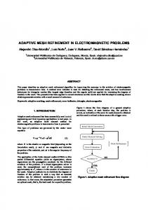
progressive display; level of detail control; more importantly, multiresolution editing. The latter is one of the most important, as details usually appear in dierent scales and require the matching of the detail scale with the level of detail of the geometry being processed. Adaptive hierarchical data structures can be used to construct a generalization of a multiresolution mesh obtained by subdivision. The mesh representation used in this work is based on [3], which presents a mesh simplication method that generates a variable resolution hierarchical structure called 4-K mesh. This method is based on simple local operators for mesh modication, which are applied in parallel to an independent set of four-face clusters. We also construct a smooth parametrization of the original mesh over the base domain, where the parametrization is dened by a composition of a sequence of mappings built during the simplication process. This approach was rst introduced by [4] and our method is based on it (a detailed description can be found in section 4.4.1). Although our method is based on [3] and [4] we can cite some characteristics that distinguish our approach from them. We build the 4-k mesh using a feature sensitive decimation process which enables us to build base meshes closer to the original one. By using 4-k meshes, our parameterization, in spite of being similar to [3], relies heavily on stellar operation which makes the process simpler than in [4]. This work relies on procedural noise generation approaches and subdivision schemes combined with the previous described techniques in order to produce rich details and also enable some sort of control over the pseudo-random appearance of the applied noise. The two main noise functions discussed here are the Perlin noise [5] and the Gabor noise [6]. The subdivision technique used here inspired by Loop's [7] scheme, which provides a nice manipulation tool when dealing with the problem of inserting band limited noise which is not compatible with the resolution or desired level of detail of the mesh. It is also a powerful tool for local manipulation as will be presented in Chapter 5. We must emphasize that we do not use Loop's approach here, but a mesh renement and smoothing scheme based on it. A full demonstration of our approach and methodology can be seen in Figure 1.1. The process described in Figure 1.1 starts with an input dense mesh with approximately 40k vertices. A decimation process then is performed, creating an adaptive hier-

1.4 Overview of the methodology

4

Figure 1.1: Steps representing our approach and methodology, where an input mesh is simplied, deformed and rened. Model obtained from [8].

1.5 Contributions

5

archical structure through successive parametrizations, reducing the number of vertices by a factor of 40. The mapping of the parameterized points can also be seen in Figure 1.1 (fourth and fth skulls). At a given resolution level (this level is user dened), a deformation is performed and a correction of the parametrization is applied (fth skull). Then, the renement process is initiated. One can notice that skulls six (11k vertices) and seven (40k vertices) are really similar, indicating that the input mesh is oversampled. All the steps and procedures mentioned previously will be explained in the following chapters of this thesis.

1.5 Contributions The main contributions of this work are: a new method based on a combination of variable resolution mesh representations, procedural noise generation and subdivision schemes for adding details to meshes with arbitrary genuses with control over the noise scales and mesh local resolution. The insertion is done in a controlled way by matching the details in the dierent scales of the procedurally generated signal (a noise) with the meshes' levels of resolution. a novel way to build 4-k meshes without relying on storing local combinatorial operations. We simply store the original vertices in the base domain and rene it by inserting the vertices in the decimation order. To achieve this, we apply a vertex degree x algorithm, which approximates the original geometry. an improvement in the 4-k base domain generation by using feature guided decimation. a new way to map details onto meshes using features and geometric properties of the mesh to guide the detail generation.

1.6 Thesis Organization This work is organized as follows: the Chapter 2 presents a review of the related works, which are the basis for the development of this thesis; Chapter 3 presents a background overview, including summary of the fundamentals and main ndings in the literature, which will serve as base to the models and methods that are presented in the next chapter;

1.6 Thesis Organization

6

Chapter 4 describes our work and its details, covering all contributions made; Chapter 5 shows the results obtained through our experiments; Finally, Chapter 6, traces future works for this research; After all chapters, we list the references cited throughout the text.

Chapter 2

Related Work

We classify the works related to the one presented here into three main categories: surface representation, procedural model or detail generation and mesh deformation. In the surface representation category, the hierarchical structures that were considered more important for this work are reviewed, focusing on techniques that provide variable resolution representations, including the ones used as the basis for the design of algorithms proposed in this thesis. In the procedural detail generation category, algorithms related to the procedural noise generation are analyzed. Many works are important, but we focus here in the two most commonly used: Perlin noise and the Gabor noise. Finally, an overview of the mesh deformation approaches are presented. These include methods based on procedural approaches and the most relevant alternatives.

2.1 Surface Representation Polygonal meshes are the main and

de facto form of surface representation used in Com-

puter Graphics. They can represent meshes of arbitrary topology, and resolve ne details when a sucient amount of polygons is used. For an extremely dense mesh, interactive manipulation is a challenge. This is due to the considerable number of operations required to modify thousands or millions of vertex, edge and/or face information. In such situations, mesh simplication algorithms can provide a possible answer [9]. One of the rst works dealing with hierarchical triangulations was presented by Floriani and Puppo [10], which consists of a subdivision scheme of the plane domain into nested triangulations and where the hierarchical structure is described by a tree. They

2.1 Surface Representation

8

also discuss details regarding hierarchical triangulations, and provide a multiresolution surface model. Later, Puppo et al. [11] presented a generalization of the multiresolution class, extending the concepts presented in [12]. This generalization introduced the idea of variable resolution structures, where an application could extract a representation of minimum size for an arbitrary LOD (level of detail) in linear time. In this work specically, we make use of a variable resolution structure called hierarchical 4-k mesh, which is a powerful representation for non-uniform level of detail. This structure is based on the

Variable Resolution 4-k Meshes introduced by Velho and

Gomes [13] and is a specialization of the general variable resolution structure. To obtain such structure a hierarchical mesh simplication process is done [3]. This representation is ideal to our work, which focus on manipulating variable resolution meshes through procedural methods. This is a direct result of the characteristics of this structure, which can code all possible mesh hierarchies that can be generated from a sequence of local modications. As presented by [11], the eectiveness of a variable resolution structure can be analyzed by three criteria: expressive power, depth and growth rate. 4-k meshes posses all these desirable properties. In Section 4.4, a detailed description of this structure is presented and for a more in-depth description we suggest reading [13]. On each step of the simplication process, a local parametrization process is performed, where the removed vertex is mapped to a lower resolution level face. In essence, this hierarchical parametrization is similar to the work presented by Lee in [4], but, as will be shown in Section 4.4.1, it has key dierences when compared to our method. Lee introduced an algorithm to compute smooth parameterizations of dense 2-manifold meshes with arbitrary topology, which is used for adaptive hierarchical remeshing of these arbitrary meshes into subdivision meshes. In [1] Maximo et al. presents an adaptive multiresolution mesh representation exploring the computational dierences of the CPU and the GPU. This work considers a dense input mesh and simplify it to a base domain, similar to the work presented in [4], but here using an atlas structure. It also uses stellar operators in order to perform both, the simplication and the renement processes. It's main objective is to show the adaptive control of the mesh resolution in CPU-GPU coupled applications. While our work is similar to Maximo's in the way the mesh representation is constructed, we can point out one key dierence. Here we used a 4-k adaptation scheme instead of 4-8 used by Maximo and this choice is explained for two reasons: rst we were not concerned with GPU processing; second, the use of feature decimation has led us to use 4-k meshes because of the distri-

2.2 Procedural Generation

9

bution of the valency of the vertices of the meshes we obtained, which made complicated the use of 4-8 meshes. Besides, in this thesis we focus in the use of 4-k structures in the problem of detail insertion. Maximo's work is also able to deal with such problem, but his approach is a more general one and not focused specically in the aspect of detail generation. As they represent a mesh as a multiresolution atlas structure that can be used as a multiresolution grid parameterization of the mesh, general geometric processing techniques can be applied. The use of the techniques proposed here is a possibility, but this requires further investigation, in particular, how to consider feature decimation in the construction of their mesh representation. Due to the characteristics of our main objective, which is detail insertion, and not the extraction of all possible representations in the adaptive hierarchical representation, we do not store local modication operations as in the classical 4-8 and 4-k mesh. On the one hand, we only store the sequence of decimated vertices in order to navigate and manipulate the structure. On the other hand, this has obliged us to devise a new way to correct the rened mesh as we reinsert the vertices, which is our vertex valency x algorithm. By doing this we made a trade o between local modication storage as a graph and procedural correction of the vertex x. More about this issue will be discussed in the description of our method in Chapter 4.

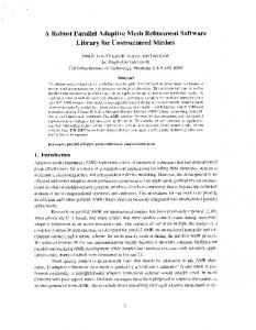
2.2 Procedural Generation Procedural methods have a great appeal and this can be explained by its characteristics. As presented by Ebert, in [14], the most important one is abstraction. In a procedural approach, every detail is abstracted into a function or an algorithm. This allows us to gain parametric control, making the manipulation of specic details an easier task, making procedural generation a powerful tool in texturing and modeling. A variety of dierent eects can be produced by procedural techniques. Among them, the most basic one, is the generation of primitives with random (or pseudo-random) parameters. A plane with a randomly generated heightmap is an example of this technique and can be seen in Figure 2.1. Also, considering pseudo-random functions, it is possible to generate noise in order to create textures and natural looking formations [5]. The process of creating organic structures, such as a tree, a snow ake or a mountain silhouette can be achieved through fractal algorithms or even L-Systems. In their book, Ebert et al. [14], outline the most important features of procedural techniques: abstraction , parametric control and exibility.


(a)

10

(b)

Figure 2.1: (a) Pseudo-random heightmap generated over a plane. (b) Resulting deformation when applying the heightmap to modify the plane geometry. In a procedural approach, any complex data is usually

abstracted into a function or

algorithm. This diers from non-procedural techniques, where all the data is explicitly specied and all complex detail of a scene is previously stored. This enables an on-they evaluation of this function or algorithm to create the desired eect, also enabling the creation of inherent multiresolution models and textures that we can evaluate to the required resolution [14]. The parametric

control is related to how the parameters represent information. These

are dened and adjusted to match certain objectives or behavior of the procedural function or algorithm, an example is a variable that denes how rough or at a terrain will be. This control allows the user to create as many as needed parameters amplifying its choices and possibilities for modeling or generating detail. The exibility of a procedural model is related to the possibility of designing an eect or structure without being bound to the real-world physics related to it. The process (algorithm or function) can capture the essence of the object being modeled and then, if necessary, insert the desired level of delity regarding the laws of physics. These characteristics draw the attention of dierent industries, such as games and movies. These are always battling to meet the expectations of the public with great concern regarding the expenses to be invested for this purpose. In order to solve this issue, the most common methodology used to take care of consumer demand has always been to essentially expand the amount of artists to create more itemized, detailed and realistic content. Nonetheless, increasing the artistic pipeline does not necessarily imply in scaling the production [15]. A potential solution for the content creation problem is the application of procedu-


11

ral techniques. These techniques have been used for over 25 years in the eld of computer graphics [14] for a wide range of applications: adding noise to existing textures and/or meshes [5], duplicate the appearance of natural materials such as marble and wood through 3D textures [16], creating and modeling life-like models of various tree and plant species [17] and generating detailed cellular textures such as skin or bark [18]. Entire procedural worlds are now possible and this is demonstrated in the MojoWorld [19] application, where assets including realistic natural features such as terrain, lakes, trees and shrubs are all generated using procedural techniques. Also, recent procedural applications have been expanded further, in order to simulate special eects including particle systems, water, and even the natural physical movements of assets [20]. Complex scenes containing many dierent models would normally take months to manually construct; now vast sections of these scenes can be created using specic procedural generation packages [21] that can generate detailed and varied models in minutes. Procedural generation is a time saving method of rapidly and eciently generating content that can help to alleviate and potentially solve the problems of escalating content creation costs [22]. There are several works that deal with the procedural generation of terrains, which is one of the most discussed application of procedural techniques [23]. Existing procedural solutions primarily apply procedural techniques to the generation of natural phenomena, but many of the same techniques have obvious applications in the generation of man-made articial phenomena. An example are cityscapes, which presents many challenges to modeling. They are rich in visual and functional complexity, and are a result of development and evolution over hundreds of years under the inuence of countless factors. Some of the major inuential factors aecting cities include population, transport, environment, elevation, vegetation, geology and cultural inuence. It is a formidable challenge for researchers and developers to create a realistic model of such a large and complex system [22]. In this scope, noise generation has always been of great importance to this end as it is one of the means to introduce randomized non-correlated features to the geometry or distribution of objects in scene. Specically, Perlin noise [5] was one of the most used and explored one. Perlin in [24], deals with the important issue of controlling the appearance of the noise. This is done through spectral control and in [24] this is achieved by a weighted sum of band-limited octaves of noise. Although, this may not be the best solution, it is only a means of controlling the power spectrum of the noise. Later, Perlin [25] improved his noise by xing discontinuities of the second order interpolation and optimizing the

2.3 Mesh Deformation

12

gradient computation. We consider noise control a key element to this work, and a noise generation approach that provides more of such control is presented by Lagae et al. [6]. He introduced a procedural noise using sparse Gabor convolution which provides accurate spectral control using Gabor kernels. Also, this approach has two qualities: it does not have the regularity and discontinuity problems of Perlin's noise function and at the same time enables anisotropic noise generation. Later, Lagae et al. in [26] presented a ltered version of the Gabor noise, where a slicing approach is introduced in order to preserve continuity across sharp edges. He also deals with the issue of keeping the anisotropic feature in a sliced solid noise. More recently, in [27], a generalization of the Gabor noise is introduced by Galerne, where a bandwidth-quantized Gabor noise with arbitrary power spectra is presented. This enables a robust parameter estimation and ecient procedural evaluation.

2.3 Mesh Deformation Mesh deformation is a challenging topic, since the techniques involved must encapsulate complex mathematical formulations into an intuitive user interface and, more importantly, must be developed to achieve eciency and robustness, allowing real-time interactions and manipulations. Shape editing has been an extremely active eld ever since the early beginnings of computer graphics and accordingly a variety of approaches exist ranging from classical splines to multiresolution techniques and space deformations. We will give only a brief overview of the principal approaches here and refer for a more general review of shape editing to [28] and [29]. Tensor product splines are nowadays the prevailing representation for surfaces in computer aided design. In many applications, surfaces are created from scratch in this representation. Spline basis functions have a number of desirable properties, e.g. local support and positive partition of unity that give linear coecients - the control points an intuitive interpretation and thus simplify subsequent editing. Conversion of large unstructured point clouds or triangle meshes as acquired by scanning devices or photometric stereo into a spline based representation is, however, dicult and still an active topic of research. Large or complex surfaces usually require tensor product spline patches with several hundreds of degrees of freedom. Except for changes to small details, the editing of such surfaces thus involves modications of many control points and is therefore often


13

tedious and troublesome. To overcome restrictions of tensor product spline surfaces, a second class of approaches [30, 31, 32] is based on what is called transformation propagation. The user initializes the editing process by selecting a subset of the surface as

region-of-interest

(ROI) R. Within this region, he then selects two further subsets: a xed subset F and a handle subset H . The points in the handle subset H are then transformed interactively by some user specied transformation (usually translation, rotation and scaling). The deformable model interactively computes positions for the remaining surface points in the region-of-interest. This general editing metaphor introduced by [30] and [33] is also used in shape editing based on deformation potentials that will be discussed below. In transformation propagation approaches, the handle transformation is propagated through the regions of interest until it reaches the xed subset F . Each point within R is transformed with an interpolation of the handle transformation and the original xed transformation at F according to some function of its distance to these regions. As demonstrated in [29] transformation propagation does not necessarily lead to intuitive deformations. Multiresolution deformation techniques decompose the original surface into a low-pass ltered coarse approximation and high-frequency details. The actual parameters of the lter can be congured by the user to select the level-of-detail of interest. Modications are then applied to the coarse version of the surface e.g. by transformation propagation or any arbitrary editing technique. Finally, the stored high-frequency details are added on top of the edited version of the coarse approximation. Approaches dier, rst of all, in the way high frequency detail is represented and fused with the edited coarse mesh. In all surface-based deformation techniques the quality of deformations is inherently linked to mesh quality. Problems in the triangulation like cracks or degenerate triangles inevitably lead to deformation artifacts. Furthermore, the speed of such methods decreases with the mesh resolution so that very high mesh resolutions result in noninteractive frame rates. Space deformation methods avoid these problems by deforming the space surrounding the object. The embedded surface is deformed by applying this space deformation to every point. Space deformations can for example be dened by tensor product splines, radial basis functions or specially designed cages around the surface in question. The complexity of the deformation then only depends on the complexity of the control structure, e.g. the number of control points or cage cells. As the actual surface mesh is not involved in the computations, space deformation approaches handle meshing problems gracefully and can equally be applied to point sets. On the downside,


14

special care must be taken to ensure sucient resolution and correct topology of control structures. Finally, another class of approaches minimizes surface-based deformation potentials for shape editing. For user interaction the same general editing metaphor is used as with transformation propagation based editing. In contrast to transformation propagation, the unconstrained surface within the region-of-interest is updated by minimizing a potential functional on the surface. Possible choices of the potential functional include linear approximations of the elastic energy discussed in Section 3.2.1. Apart from these, mesh editing methods based on dierential representations, as they have become very popular in the last years, also naturally lead to deformation potentials and can therefore be subsumed into this class of approaches. In our scope, an important work is presented by Velho in [34] where he introduce a framework that integrates procedural shape synthesis on a modeling system. This is done using multiresolution analysis through surface subdivision based on Catmull-Clark [35]. This is a key dierence in relation to our work, in which a variable resolution structure is used, where we guarantee feature preservation in the base domain. This last characteristic has some advantages, enabling, for instance, the creation of level of detail structures with better quality. Regarding feature guided mesh editing, Biermman [36] describe a method to introduce sharp features and trim regions on a surface. Similarly to Velho's work, he uses a multiresolution representation also using Catmull-Clark subdivision scheme. The subdivision surfaces mentioned before, are dened by progressive renement rules applied to an initial polygonal mesh (in some cases a base domain). For example, CatmullClark subdivision inserts new vertices at the center of each edge and face, and then displaces the vertices based on simple linear weights. Considering a initial quad-mesh, this process converges to a bi-cubic B-spline surface dened by this mesh [37]. However, this scheme lacks the adaptive feature of a variable resolution representation. In this chapter we presented the most important references that relates to our problem and solution, including relevant surface representation methods, procedural detail generation algorithms and mesh deformation approaches. In the next Chapter, all the necessary background information, needed for a better understanding of the rest of this thesis, will be presented. Including object representations, parametrization and procedural noise functions.

Chapter 3

Background

This chapter presents the basic information needed to the comprehension of this thesis. The main objective is to expose the technical and theoretical background, establishing the basis for the methodology that will be described to solve the problem. Here, we will focus on the following topics: representation of geometric data using meshes and the types of geometric and topological operators used by the majority of the problems of geometry processing; construction of topological data structures in variable resolution; simplication strategies, parameterization methods and procedural noise functions, considered in the methodology we propose.

3.1 Object Representations In geometry processing, identifying the most prominent set of operators by which the computation is dominated is paramount to every problem. This leads to the denition of the most appropriate data structure used to support the ecient implementation of these operators. In this work, all objects can be approximated by polyhedral surfaces [38], which can be understood as geometric realizations of 2D meshes, which are usually used to describe the topology of a subdivision of two-dimensional domains.

3.1.1 Polyhedral Meshes According to algebraic topology, a mesh M can be dened as a pair (K, V ), where K is a simplicial complex that represents the connectivity of vertex, edges and faces, determining the topological type of the mesh. Thus, V is a set of vertex positions {v1 , ..., vn } , vi ∈ R3 , which denes the mesh geometry.

3.1 Object Representations

16

A simplicial complex K is a vertex set {1, ..., n}, composed by a nite number of simplexes, which are non-empty subsets of these vertices. 0 − simplexes {i} ∈ K are vertices, 1 − simplexes {i, j} ∈ K are edges and 2 − simplexes {i, j, k} ∈ K are faces (triangles). In general, n − simplexes are polytopes with n+1 vertices. One of the main mesh types used in geometry and graphics processing is the triangle mesh. Triangles have several properties that justify the previous statement. One of the most important, among such properties, is the ability to dene coordinate systems in the mesh structure using barycentric coordinates. This allows the construction of parametrizations for surfaces with disk topology, solving both the problem of representation and reconstruction.

3.1.2 Geometric Operators Operators on Meshes Since polygonal meshes are piecewise linear surfaces, the approximation of dierential properties of the underlying surface can be obtained from the mesh data. This is due to the fact that meshes can be interpreted as piecewise linear approximations of smooth surfaces. The following denitions present the most basic operators and are based on Botsch's et al. [39].

3.1.2.1 Normal Vectors Calculating normal vectors to either faces or vertices, is critical for most methods of geometry processing. For triangles described by vertices (xi , xj , xk ), the normalized normal vector can be obtained by equation 3.1.

n(T ) =

(xj − xi ) × (xk − xi ) k(xj − xi ) × (xk − xi )k

(3.1)

The normal vector at a vertex v can be calculated by a weighted average of the normals for each incident face n(T ) in a neighborhood N1 of v , with weights given by α(T ). P T ∈N1 (v) αT n(T )

n(v) = (3.2)

P

T ∈N1 (v) αT n(T ) Botsch et al. [39] discuss several possibilities for weights. Here we follow them closely: Uniform (α(T ) = 1) : it is ecient, but produces counter-intuitive results, since it does not consider edge lengths, triangle area or angle at the vertex. In other words,


17

it does not consider the geometry of the mesh. Based on the triangle area (α(T ) = AT ): also ecient, but can also lead to counterintuitive results(Figure 3.1). Based on the incident angle of the triangle (α(T ) = θT ): corresponds to mean values computed in small geodesic disks; generally produces the best results.

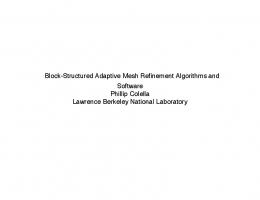
Figure 3.1: Dierent methods are used to compute per-vertex normals. Using constant and area weights yields the result in the center, while the results using angle weights can be seen on the right. Figure obtained from the book Polygon Mesh Processing [39].

3.1.2.2 Gradients The discrete gradient of a piecewise linear function fi dened at each vertex vi , can be computed from Equation 3.3. In Equation 3.3, fi = f (vi ) = f (xi ) = f (ui ) and u = (u, v) is an ordered pair in the conformal parameter space.

∇f (u) = (fj − fi )

(xi − xk )⊥ (xj − xk )⊥ + (fk − fi ) 2AT 2AT

(3.3)

3.1.2.3 Discrete Mean Curvature The Laplace-Beltrami operator presented by Taubin [40] (see Equation 3.4), when applied to the coordinate xi of a vertex vi , yields a discrete approximation of the mean curvature.

∇f (vi ) =

1 2Ai

X vj ∈N1 (vi )

(cot αi,j + cot βi,j )(fj − fi )

(3.4)


18

Therefore, it is possible to set the absolute mean curvature as:

H(vi ) =

1 k∆x + ik 2

(3.5)

For the Gaussian curvature, it is possible to use the following expression, based on the Gauss-Bonet theorem, where θj is the angle of the incident triangles of vi :

 K(vi ) =



1  2π − Ai

X

θj 

(3.6)

vj ∈N1 (vi )

Given the formulas for the discrete mean and Gaussian curvatures, it is possible to compute the principal curvatures k1 and k2 from the formula:

k1,2 = H(vi ) ±

p H(vi )2 − K(vi )

(3.7)

To end this section, we can mention the following works that present, in greater depth, the various discrete operators and their properties and characteristics, such as convergence and robustness: [41, 42, 43, 44], and [45].

3.1.3 Topological Data-structures The representation of an object by a polygonal mesh is the problem of describing a continuous model by a nite set of primitives. This process must guarantee that topological and geometrical characteristics of the original object are maintained. There is also, when dealing with the computational side of this problem, the implementation issues related to data structure denitions, in order to store such information. The main issue to be dealt with is the denition of operations supposed to be performed on the models, which can be implemented as algorithms associated with such data structures. In the literature, there are many works that deal with this matter, as seen in Chapter 2, where each method seeks to meet a set of properties that vary according to the application or problem which it is intended to deal with. Nevertheless, there exists key requirements that every structure for mesh representation must be conformed with: minimize redundancy; ecient use of storage space; ability to respond to spatial and topological queries eciently; ability to describe levels of detail and hierarchy relationships.


19

Velho et al. in [38], makes a parallel between a structure for mesh representation and a geometric database, due to the need to eciently respond to geometrical and topological queries. This is of major importance when designing such data structure, where queries like boundary of a face or a vertex star must be answered in optimal time. Indeed, these are the most common operations that can be applied to a mesh structure, but there are other ones that must be considered, for example, renement and smoothing operations on surfaces, which are the result of subdivision processes ([7, 46, 47, 48, 49]); application of discrete dierential operators, application of topological operators; and operations to manipulate levels of detail (local changes) ([10]). In the literature, one can nd many dierent topological data structures, usually proposed to solve a specic problem or problems that incorporate a variety of properties expanding precursor data structures. Although initially topological data structures have been created in order to represent subdivisions and objects with the topology of the sphere, these have evolved to deal with more complex problems. Considering the most inuential works related to the construction of such structures, we can name the Winged-Edge Baumgart [50] and Mäntylä's Half-Edge [51]. Also, others that should be cited in the text, are: the Corner Table [52], a compact and ecient structure to describe triangulations based on indexes and integer arithmetic operations; the Lage's [53] CHE and Gurung's [54] sQuad.

3.1.4 Representation of Meshes at Multiple Levels of Detail In this thesis, the necessity of representing objects at dierent levels of detail is paramount. Also, it is important to have the ability to manipulate objects considering a greater level of detail in some areas than in others. This is also a concern in the geometry processing area, leading to an investigation of data structure algorithms that can support such functionality. Due to the characteristics of the concept of level of detail, one can create a relation with the notion of hierarchy. Thus, according to Velho and Gomes in [13], hierarchical data structures are a natural option to give computational support to representations with multiple levels of detail. Still according to them, hierarchical data structures are the materialization of abstraction mechanisms used to deal with complexity and relationships between entities at dierent levels, where these relations depend on the application and the context of the problem.


20

Velho and Gomes dene a mesh hierarchy as a sequence of meshes H = M j , j =

1..., n − 1, such that the size of a mesh M j monotonically increases with the index j . It is important to mention that, the mesh hierarchy must capture and maintain the dependency relationships between faces of two consecutive levels j and j+1, whose support overlap. These are constructed through operations denominated

local movements, which

can both rene and simplify an initial mesh. Examples of operators that can perform local movements are stellar

operators. The type of the local modication operator denes

the properties of the hierarchy, which can be adaptive or non-adaptive.

3.1.4.1 Non-Adaptive Hierarchical Structures A non-adaptive hierarchical structure denes a single mesh hierarchy [13]. Multiresolution and Progressive Meshes are typical examples of non-adaptive hierarchical data structures. On the one hand, multiresolution meshes are characterized by the fact that operations are applied in parallel on a whole set of independent regions covering the whole mesh, changing the resolution globally. On the other hand, progressive meshes apply these modications sequentially to each specic region separately. A tree data structure is used to capture the structure and relationships of a multiresolution mesh, which is usually built via multiresolution renement(Figure 3.2).

Figure 3.2: Tree representation of an enclosing hierarchy. Figure obtained from [10]. Dierently, on progressive meshes, the corresponding data structure is a list data structure which is usually constructed via simplication.


21

3.1.4.2 Adaptive Hierarchical Structure Adaptive hierarchical structures construct a family of mesh hierarchies. An example of this structure is a

variable resolution mesh and the data structure for representing it

is a DAG (Discrete Acyclic Graph). Such structures can be created either by rening or simplication processes, also known as decimation. In such data structures, local modication operations are applied to independent region sets, but they do not necessarily cover the entire mesh, with the constraint that the edges dening the boundary of the region must not be changed, generating the concept of minimally compatible local changes. In the sequel, three hierarchical structures for meshes are presented, two adaptive ones and one non-adaptive structure.

Hierarchical Triangulation Floriani and Puppo [10] introduced the idea of hierarchical triangulations, which is an example of multiresolution hierarchical structure. The proposed denition for this triangulation is a triple T H = (T r, E, l) representing a tree, where T r are the nodes corresponding to a sequence of triangulations, E is a set of labeled arcs that connect the dierent triangulations according to the hierarchical relationships and l is a labeling function. Figure 3.2 shows exactly this type of structure. Formally dened as: T r = {τ0 , τ1 , ..., τh } , ∀j = 0, ..., h, τj = {Vj , Ej , Tj } with Tj > 1 and ∀j > 0 there is only one triangle tj ∈ Ti , for some i < j , tj = D(Tj ) where D(Tj ) is the domain of the triangulation τj , dened by the union of the triangles in Tj . E = (τi , τj ), τi , τj ∈ Tr , ∃tj ∈ Ti , tj = D(Tj ) where E is a set of labeled arcs connecting two triangulations τi and τj where τj is the renement of a triangle in

Ti . l : E → ∪{i=0,...,h} Ti , l(τi , τj ) = tj if tj ∈ Ti and tj = D(Tj ). Every triangle in l(E)

macrotriangle, while triangles that do not belong to l(E) are considered simple triangles. is a

The data structure used to code a hierarchical triangulation is based on the Edelsbrunner's graph of incidence [55]. Thus, let GI = {GI0 , GI1 , ..., GIh } be a collection of


22

incidence graphs. Hence, a hierarchical graph of incidence is a triple GIH = {GI, Eg , lg } where: Eg = {(GIj , GIi )|(τi , τj ) ∈ E} lg : Eg → ∪{i=0,...,h} N Ti , lg (GIj , GIi ) = ηT−1 (l(τi , τj )) To search for the neighbors, the structure proposed by Floriani stores a set of arcs linking neighbors in the structure, which are called strings. The construction of the hierarchical graph of incidence is presented in details in [55].

4-k Meshes A variable resolution 4-k mesh, proposed by Gomes and Velho, is a hierarchical structure that contains at each level approximately half of its vertices of valence four and other vertices of arbitrary valence k . Variable resolution triangulations are based on the concept of

ible local changes.

minimally compat-

The descriptions presented here are based on Gomes and Velho's

work [13].

Denition 1 (Minimally Compatible Local Changes).

"A minimally compat-

ible local change W (K i ), applied to a submesh M i ⊂ M of a mesh M = (V, E, F ), is a substitution of M i by W (M i ), which satises the following properties: Edges of the border of M i are not altered. Interior edges of M i are replaced by new edges." The submeshes K i and W (M i ) are the pre-image and image of the local modication operator W .

Denition 2 (Compatible mesh sequence).

"A mesh sequence {M 0 , M 1 , M 2 , ...,

M n }, generated by applying a sequence of operators {W1 , W2 , ..., Wn }, starting with a initial mesh M 0 , generates a compatible mesh sequence. The sequence generated by this approach is given by {M 0 , W1 (M 1 ), ..., Wn (M n )} where M j =

Wj−1 (Wj−2 (...W1 (M 1 ))), j > 0".


23

A fundamental dierence between a mesh structure with variable resolution and a multiresolution structure is that, given a intermediate mesh M m and two compatible operations Wi and Wj , it is possible to generate two new distinct meshes M m+1 = Wi (M i ) or M m+1 = Wj (M j ), M i , M j ⊂ M m . The purpose of a variable resolution structure is being able to code all possible mesh hierarchies through a valid sequence of minimally compatible local changes.

Denition 3 (Variable resolution mesh).

"A mesh M = (M 0 , W, ≤) is dened

by a initial mesh M 0 , a set of operators W = {W0 , W1 , ..., Wn } and a relation of partial order ≤, dened over the operators satisfying dependency and non redundancy properties. Dependency implies that, if f ∈ Fi , on the pre-image M i of Wi (Mi ) and also belongs to Wj (M j ) then Wi precedes Wj . The non-redundancy implies the fact that, if f ∈ Fi of Wi (Mi ), then f ∈ / Fj of Wj (Mj ) for all i 6= j ". The 4-k structure was proposed by Gomes and Velho through the specialization of the model described by Puppo for triangulations based on a 4-8 mesh, which itself is based on Laves tilings[4.82 ]. As will be presented in the next section, on regular 4-8 meshes, vertices always have valency 4 or 8, on semi-regular 4-8 meshes it is possible to nd isolated extraordinary vertices, and on quasi-regular 4-8 meshes there are extraordinary vertices that are not necessarily isolated. The 4-8 meshes are renable and it is possible to build a multiresolution structure based on subdivision operators, which can be quaternary or interleaved binaries, the latter being the most widely used. The multiresolution representation for 4-8 meshes is done through a quaternary or binary tree structure, depending on the operator type. On the other hand, 4-k meshes are hierarchical structures, with variable resolution, in which approximately half of the vertices have valency 4 and the other half has valency

k . The local modication operators are restrained to clusters of two triangles forming a convex structure and can be of two types: edge split and edge swap(ip) (see Figure 3.3). In the implementation of the 4-k mesh, a combination of elements of edge and face types are used. The edge split operator is a renement operator, which makes the edge that separates two faces to be subdivided, making two faces give rise to four new faces. Therefore, the data structure for edges must maintain a pointer to the two faces thereto adjacent, and each face must maintain two pointers to their faces' children, which in turn points to the parent faces. The edge swap operator does not subdivide edges, then one of the pointers of the face structure is kept as null.


(a)

24

(b)

Figure 3.3: Stellar operators:(a) Face split and face weld. (b) Edge split and edge weld. An example of variable resolution mesh structure is the 4-k structure. The 4-k meshes have good expressiveness power, derived in part of some properties it shares with 48 meshes. Besides that, it is possible to easily implement, in the structure, variable resolution query operations and adaptive mesh extraction.

4-8 Tessellations and Meshes A 4-8 tessellation is a renable tiling. It exploits the self-similarity subdivision characteristic of a [4.82 ]. Therefore, it is possible to construct a multiresolution 4-8 tessellation using renement. In this structure we can name some advantages: The [4.82 ] Laves tiling is a triangulated quadrangulation, thus it combines the advantage of both triangular and quadrilateral meshes; They can generate adaptive tessellations in variable resolution, due to the support of both uniform and non-uniform renement; Both available construction methods are intuitive and easy to implement. There are two alternative construction methods: quaternary subdivision and interleaved binary subdivision. The quaternary subdivision renement algorithm for a given 4-8 mesh M = (V, E, F ) is shown in Algorithm 1 and is represented in Figure 3.4(a):

Algorithm 1.

Quaternary Subdivision

1. Split all edges e ∈ E at their midpoints m;


25

Figure 3.4: (a) Binary subdivision. (b) Quaternary subdivision. Image based on an image presented in [48] 2. Subdivide all faces f ∈ F into four new faces, linking the degree four vertex,

v ∈ V4 , to the midpoint m of the opposite edge. 3. Link m to the midpoints of the two other edges. The interleaved binary subdivision is as follows and can be seen in Figure 3.4(b):

Algorithm 2.

Interleaved Binary Subdivision

Repeat two times: 1. Split all edges e = (vi , vj ) ∈ E that are formed by two vertices of valence 8,

vi , vj ∈ V8 ; 2. Subdivide all faces f ∈ F into two sub-faces, by linking the degree 4 vertex,

v ∈ V4 , to the midpoint m of the opposing edge. A multiresolution 4-8 mesh can be represented through a tree structure of triangles. Depending on the type of renement used, this tree is a binary or quaternary one. We have three types of 4-8 meshes: Regular 4-8 meshes, Semi-Regular 4-8 meshes and Quasi-Regular 4-8 meshes. A

Regular 4-8 mesh

is homogeneous simplicial com-

plex that has the same connectivity of a [4.82 ] tiling [13], meaning that all vertices in this representation has valence 4 or 8 and are all regular vertices. Another important characteristic is that all valence 4 vertices have only valence 8 neighbors(1-neighborhood), and all valence 8 vertices have neighbors consisting of vertices with alternating valences 4 and 8. A

Semi-Regular 4-8 mesh is a tessellation that has isolated extraordinary vertices,

whose valence is dierent than 4 or 8. Usually these meshes are created from a coarse irregular mesh by applying a semi-regular 4-8 renement method that introduces only

3.1 Object Representations regular vertices [56]. Finally, a

26

Quasi-Regular 4-8 mesh is a tessellation where, dier-

ently from the previously mentioned representation, irregular vertices are not guaranteed to be isolated.

3.1.5 Simplication A mesh simplication describes a class of algorithms that has the aim of transforming a mesh into another with fewer faces, edges and vertices [57]. There are two ways of dening this problem: a rst approach that aims to generate a mesh of xed size and a second one that seeks the best geometric approximation. Solving the simplication problem is also the starting point of the solution of other problems, like the construction of hierarchies, which is part of the proposal of this work. The optimal solution of the simplication problem is not always possible, since it is NP-Hard, thus interactive heuristic methods were developed in order to achieve a dened criterion. This is done by applying a simplication operator onto the mesh. In the literature, there are several approaches regarding the mesh simplication. Initially, as mentioned in [39], the complexity reduction can be done as a one-step operation or by an interactive process. These approaches are dened, by Paul Heckbert in [58] as: vertex clustering algorithms, incremental decimation algorithms, resampling algorithms and mesh approximation algorithms. Also, an important observation is that all simplicial complexes can be transformed into a simpler one, through a simple sequence of

edge swap and edge collapse operators,

allowing the denition of simplication operators that preserve the mesh topology, a major concept to this work.

3.1.6 Simplication based on the quadric error metric In order to provide a powerful, yet simple approach for a mesh simplication, Garland and Heckbert introduced an algorithm based on the vertex pair contraction [58]. This is one of the most common methods and is dened by selecting two vertices v1 and v2 , and performing a contraction operation, where both vertices are moved to a new position

v . Then, all incident edges connected to v1 and v2 are removed. Any face that becomes degenerated is removed, guaranteeing the model consistency. The success of the pair contraction operation directly depends on the choice of which


27

vertex pairs should be contracted at each simplication step. Garland and Heckbert introduced a quadric error metric, that is associated to each pair, this gives an ecient way to estimate the geometric error between the original and simplied surfaces [3]. Specifically, for each vertex vi , a symmetric matrix Q, of order 4 × 4, that encodes a quadric surface, and the error measured in vi is given by the quadric form ∆vi = viT Qvi . Thus, to determine which pair to be chosen, we dene the cost of the contraction operation of two vertices (v1 , v2 ) → v by the form ∆v = v T (Q1 + Q2 )v , where Q1 and Q2 are the quadrics associated to v1 and v2 respectively. This algorithm has useful properties, given the local nature of its modication operator. It is possible, for example, to generate a sequence of models (Mn , Mn−1 , ..., Mg ), based on a certain level of simplication, that can build a progressive mesh structure. This idea is really similar to Hoppe's algorithm dened in [9]. The simplication algorithm can be resumed in the following pseudo-code:

Algorithm 1.

Simplication based on the quadric error metric

1. Determine all Qi matrices for all initial vertices vi ; 2. Select all valid pairs {typically all vertices connected by an edge}; 3. Determine the optimal vij positioning of each contraction pair vi , vj , considering T the contraction cost of each pair is given by vij (Qi , Qj )vij ;

4. Insert all pairs into a

heap structure, where the key will be dened by the

contraction cost; 5. Iteratively remove each pair (vi , vj ) associated with the lower

heap cost and

update all costs of pairs related to v1 .

3.1.7 Simplication based on four-face clusters As it will be seen in Chapter 4, in this work we use a simplication algorithm denominated four-face clusters mesh simplication [3]. This algorithm focus on removing vertices that has a valence equal to four. In its rst step, all vertices of the mesh are associated with a removal cost. The denition of this metric is based on the conguration of the simplication operator, which is a combination of edge swaps and degree 4 vertex removal (the vertex removal can be achieved through a stellar

edge-weld operation as Figure 3.6 shows). Thus, the error E(v), which is the


28

Figure 3.5: Four face cluster. result of the removal of the vertex v , is computed as the sum of costs of performing the mentioned operations, as described in Equation 3.8:

E(v) = αC(v) + βS(v),

(3.8)

where C(v) is the cost of removing the vertex v and S(v) is the cost of edge swaps necessary to make v a vertex of valence four [3]. This is equivalent to the vertex pair contraction cost used by Garland and Heckbert [58], meaning that, both, C(v) and S(v) are measured following Garland and Heckbert quadric error.

Algorithm 2.

Simplication using four-face clusters

1. Order all vertices based on a quality criteria; 2. Select an independent set of four-face clusters that covers most of the mesh; 3. Simplify the four-face clusters using

edge swaps and removal of vertices with

degree equal to four.

Figure 3.6: Edge contraction operation using edge swaps and edge weld.

3.2 Parametrization

29

This algorithm performs the sequence of operations in parallel, thus, to cover most of the mesh, Velho and Gomes in [3] introduced a cluster marking strategy, that creates an independent set of face clusters. To achieve this, vertices are st stored in a priority queue ordered by the error E(v). While the queue is not empty, the rst vertex (associated with the lowest error) is removed, and if it is not marked, a sequence of edge swaps is applied to make the degree of v equal to four. The vertices on the star of the cluster surrounding

v are marked to allow the construction of an independent set. Finally, the third step of the algorithm, all vertices in the center of the independent sets are removed in parallel, generating one level of simplication.

3.2 Parametrization As presented by Botsch et al. in [39], the notion of parametrization attaches a geometric coordinate system to an object, which facilitates the conversion from one mesh representation to another. There are several applications of a mesh parametrization, such as: texture mapping, re-meshing algorithms and conversion from one mesh representation to an alternative one. Parametrization is of major importance to this work, due to the possibility of transforming complex 3D modeling problems into a 2D space where, usually, they are easier to solve. Dening it more formally as presented in [39]: "a parametrization of a 3D surface is a function putting this surface in one-to-one correspondence with a 2D domain." Parameterization methods belong to two main classes: local parametrizations which build the parameterization considering only the local aspects of the surface and the global parameterization that works on it as a whole. The description of all these methods is beyond the purpose of this thesis and here we only present two examples of such methods, the Floater's barycentric parameterization [59] and the Duchamp's parametrization based on conformal mapping [60].

3.2.1 Triangle Mesh Parametrization Triangle surfaces can be dened by a mesh M and a set of positions p1 , ..., pn . The mesh

M is dened by the triplet (V, E, T ), where V is a set of vertices, E is a set of edges and T is a set of triangular faces. These are naturally parameterized using piecewise linear functions, whose pieces, in this case, are related to the triangles of the surface. This associates to each point p an ordered pair u, v in the parameter space. At a given point

3.2 Parametrization

30

(u, v), in the parameter space, the parametrization is given by:

x(u, v) = αpi + βpj + γpk

(3.9)

where pi , pj and pk are the the vertices of the triangle t ∈ T , that contains the point (u, v), and α, β and γ are barycentric coordinates in relation to t. Also, in order to guarantee a valid parametrization, the image of the surface in the parameter space must have no self-intersections.

3.2.2 Barycentric Parametrization The barycentric map is one of the most used methods in the literature for constructing a parametrization of a triangulated surface [39]. It was proposed by Floater [59] and is based on Tutte's theorem [61], from Graph Theory. The theorem states the following:

Theorem [61].

"Given a triangulated surface homeomorphic to a disk, if the (u, v)

coordinates at the boundary vertices lie on a convex polygon, and if the coordinates of the internal vertices are a convex combination of their neighbors, then the (u, v) coordinates form a valid parameterization (without self-intersections)." The second condition of this theorem, as presented in [39], is expressed mathematically by:

X ui uj ∀i ∈ {1, ..., Nint } : −ai,j ai,j = vi vi j6=i

(3.10)

where the vertices are ordered such that {1, ..., Nint } correspond to the indexes of the inner and vertices {Nint + 1, ..., N } are the indexes of the vertices of the border. Furthermore, the coecients ai,j are dened according to the following rule:

ai,j > 0, if vi and vj are connected by an edge, ai,i = −

P

j6=i

ai,j

ai,j = 0, otherwise. Thus, the solution of the parameterization problem can be obtained by solving the following system, whose solution sets the coordinates in the parameter space of the interior

3.2 Parametrization

31

vertices, once determined the coordinates of the vertices of the edge.

∀i ∈ {1, ..., Nint } :

 N int  X    ai,j uj = ui = −   j=1 N int X

     

ai,j vj = vi = −

j=1

N X

ai,j uj

j=Nint +1 N X

(3.11)

ai,j vj

j=Nint +1

3.2.3 Parametrization Based on Conformal Mapping The idea of parametrization is related to the problem of dening and computing a good map between two surfaces. A straight forward approach is to nd a map that minimizes angular distortions, leading to the preservation of local surface geometry. Hence, a natural choice are conformal maps. These are tightly related to complex analysis. It relies on the conformality condition, which denes a criterion with enough rigidity to oer good extrapolation capabilities that can compute natural boundaries [39]. In Lee et al. [4], a conformal mapping z a is dened, which minimizes the distortion metric to map the neighborhood of a vertex to the plane. The advantages of a conformal mapping are that it always exists from any surface with a disk topology to a 2D planar domain, which is one-to-one, onto, and angle preserving. According to Lee et al. [4], a conformal mapping is dened as follows: Let {i} be a vertex to be removed. Cyclically enumerate the n vertices that belong to the 1-ring

N {i} = {jk |1 ≤ k ≤ n} so that {jk−1 , i, jk } be a triangle of the original triangulation and such that j0 = jn . A linear piecewise approximation of z a is given by µi , which is dened for {i} and its neighbors in N {i} according to the following expression:

µi (pi ) = 0 µi (pjk ) = rkα eiθk α where:

(3.12)

3.3 Procedural Noise Functions

32

rk = kpi − pjk k θk =

k X

∠(pjl−1 , pi , pji )

(3.13)

l=1

a = 2π/θn When the vertex is an edge vertex, the mapping is a semi-disk and, therefore, a =

π/θn , assuming that j1 = jn and θ1 = 0.

3.3 Procedural Noise Functions Procedural noise functions are widely used in Computer Graphics due to its ability to add rich visual detail to synthetic images, what has always been one of the major challenges of this research area. Furthermore, procedural noise functions have many desirable qualities, such as: fast evaluation of complex patterns in real-time; it has a very low memory cost, which is ideal for compactly generating complex visual detail; parametrization, meaning that a large variety of patterns can be created with a suitable set of parameters; independent evaluation, where every point can be processed independently and in parallel, making this property of great importance when working in a massively parallel environment, like modern GPU's systems [62]. According to Lagae et al. in [62], a procedural noise function is a "procedural technique

for simulating and evaluating noise ". Thus, a denition of noise is needed, which is also presented by the same work: "A noise is a stationary and normal random process. Control of the power spectrum is provided, either directly, or through the summation of a number of independent scaled instances of (typically band-limited) noise." This noise description is based on the various denitions from random process and Fourier analysis described in [63, 64]. Also, the main purpose of this denition is to summarize the properties of most existing noise functions and not dene how these were designed. The next sections follow the same classication presented in [62].


33

3.3.1 Lattice Gradient Noises A noise generated by the interpolation of values and/or gradients, which are specied at the point of an integer lattice is called lattice gradient noise. Considering this denition, the rst noise that comes to mind is the Perlin noise, which is one of the rst and most successful procedural noises.

3.3.1.1 Perlin Noise Considering an integer cubic lattice in Figure 3.7, Perlin noise determines the noise of a point p computing eight pseudo-random gradients, one for each of the nearest vertices and then proceeds with an interpolation, dened by a spline function. The interpolant must guarantee a continuous noise derivative, so Perlin chose a quintic polynomial, an hermite curve function of the form:

f (x) = 6x5 − 15x4 + 10x3 .

(3.14)

This function has both rst and second derivatives of 0.0 at 0.0 and 1.0, ensuring C 2 continuity. In order to create a pseudo-random selection of the gradient vectors, lattice points are hashed by successive application of a pseudo-random permutation to the coordinates and the result is used to choose a gradient from an array. The set of gradients consists of the 12 vectors dened by the directions from the center of a cube to its edges [25]. In three dimensions, there are eight surrounding grid points. A trilinear interpolation is required to combine their respective inuences (linear interpolation in each of three dimensions).

Figure 3.7: Three dimensional example of eight surrounding grid points [16].


34

Thus, the noise of a point p is given by the function

N (p) =

+∞ X

(3.15)

ai ∗ fN (f i ∗ p),

i=−∞

where the stochastic function fN is a procedural noise as described earlier, a is the amplitude and f is the principal frequency which is related by a factor of two. An example of the appearance of this noise can be seen in Figure 3.8.

Figure 3.8: Example obtained performing a 2D Perlin noise. In Figure 3.9, we can see the denition of amplitude and frequency. For example, given a sinusoidal wave (Figure 3.9 (a)), the amplitude is dened as the wave height and the frequency as 1/wavelength. Considering now a noise function, the amplitude can be dened as the dierence between the maximum and the minimum this function could achieve. In this case, the wavelength is the distance from one point to another and the frequency relation remains the same.

(a)

(b)

Figure 3.9: (a) Amplitude and frequency denition on a sin wave. (b) A noise function example. Figure recreated from [65]


35

3.3.1.2 Other Lattice Gradient Noises There are several other noise functions based on lattices. For instance, in [66] a lattice convolution noise is presented, which uses a non-integer lattice, represented by a more densely and evenly packed grid, based on sphere packing. In [67] simplex noise is introduced, which is based on a simplex grid. Perlin and Neyret [68] presented ow noise, that deals with time-varying ow textures. We can also name, curl noise [69] and better gradient noise [70]. A more in-depth description of the many dierent lattice noises can be found in [62].

3.3.2 Sparse Convolution Approaches Sparse convolution noises use other methods to generate noise that are not based on a regular lattice of pseudo-random number (PRN). Specically, noise is generated as the sum of randomly positioned and weighted kernels.

3.3.2.1 Sparse Convolution Noise This method of generating noise involves taking random samples from a set of PRNs and ltering. Control over the power spectrum is provided in the lter parameters. The term sparse here is related to the random sampling of the PRNs, which is considered a sparse form of white noise. One draw back to this method over a lattice convolution noise is that the search space is increased for each call of the algorithm, which is computationally expensive. Aiming for a better control over the noise power spectrum, Lewis [71] introduced the sparse convolution noise, where a three dimensional noise is synthesized by the convolution (∗) of a three dimensional kernel h with a Poisson noise process γ . Lewis presents an extensive mathematical framework regarding this in [71]. We strongly recommend it in order to better understand the following sections. The following noise equation is presented in his work:

f (p) = h ∗ γ(p)

(3.16)

This Poisson process consist of impulses of uncorrelated intensity ak distributed at uncorrelated locations pk in space, which Lewis calls sparse white noise [71]:

γ(p) =

X

ak δ(p−pk ) ,

(3.17)


36

where pk is the location of the k th impulse and δ(p−pk ) = (x − xk , y − yk , z − zk ). For the function h, Lewis proposed a smooth cosine kernel presented in Equation 3.18, but, according to [72], this function has the problem of generating a second derivative at

d = 1 that is dierent from zero: h001 (1) = π 2 /2. This can be problematic in specic applications, such as hypertexturing generation, which needs to enforce C 2 continuity in order to create smooth surfaces. Regardless, the synthesis proposed by Lewis has a low computational cost without requiring sampling. Also, the noise quality can be manipulated by varying the Poisson process [71].

h1 (d) = (1 + cos(π ∗ d))/2, (|d| ≤ 1).

(3.18)

Lewis procedurally evaluates sparse convolution noise by introducing a grid, and generating the positions and weights of the kernels in each cell on the y. The grid reduces the evaluation of the noise to the grid cells close to the point of evaluation. The convolution integral can then be simplied to a basic summation over the impulses, this is due the impulsive nature of the noise, leading to the following equation:

f (p) =

X

ak h(p − pk ).

(3.19)

3.3.2.2 Spot Noise Spot noise is unique in that it shares properties of both sparse convolution noise and explicit noise. It is particularly useful for mapping textures to parametric surfaces as well as generating textures over curved surfaces [73].

3.3.2.3 Gabor Noise This method follows the similar idea of convolution, but is unique in its choice of kernel. One of the drawbacks to sparse convolution noise is that more often than not a poor kernel is generated that reveals structure in the noise; violating the ideal noise requirements. Gabor noise solves this problem by using a kernel that is a combination of a Gaussian curve and a sinusoidal curve, both in two-dimensions. Considering these characteristics, Lagae [6], proposed an anisotropic noise with accurate spectral control, which is able to provide a setup-free surface texturing. This noise is achieved by a sparse Gabor convolution which is an extension of the previously presented


37

sparse convolution noise. A band-pass Gabor noise presented in [6] is dened as:

N (p) =

X

(3.20)

wi g(Ki , ai , F0,i , ω0,i ; p − pi ),

i

where wi are the random weights, K represents the amplitude, ai is the bandwidth, F0 and ω0 are the frequency and the orientation of the cosine in the kernel as presented in Equation 3.21 and represented in Figure 3.10. g is the Gabor kernel proposed in [6]. It is possible to visualize that we have the same options to manipulate the Gabor noise as done with the Perlin noise. Also, the random positions pi are distributed according to a Poisson process with mean λ. In this context g is dened as 2 |p|2

g(p) = Ke−πa

(3.21)

cos [2πF0 (px cos ω0 + py sin ω0 )] ,

Basically, the kernel is a multiplication of a circular Gaussian and a cosine. The anisotropic feature of the Gabor Noise is paramount to the generation of detail aligned or guided by the features of a mesh as it will be shown later in this thesis.

(a)

(b)

(c)

Figure 3.10: (a) Gaussian. (b) Cosine. (c) Gabor Kernel. Figures obtained from [6] In this chapter an extensive review of techniques covering representation of geometric data, topological operators, topological data structures for variable resolution, simplication strategies, parametrization methods and procedural noise functions was presented. In the following chapter our method will be presented, which utilizes most of the techniques described herein.

Chapter 4


In this chapter we describe our method for mapping procedurally generated details onto arbitrary meshes. We start by posing a formulation for the problem we will solve in section 4.1. Later, in section 4.2, we describe the methodology used to solve the problem and, in section 4.3, we outline an overview of the method. In sections 4.4, 4.5 and 4.6, we describe each of the main steps of the method: section 4.4 describes the construction of the hierarchical parameterized mesh representation, section 4.5 describes the detail mapping approach using the data structure and nally, section 4.6 explains the adaptive renement step used tho reconstruct the mesh after detail and deformation are applied to the input mesh.

4.1 Problem denition Given a surface S represented by a mesh M = (V, E, F ) compute a new mesh M 0 (V 0 , E 0 , F 0 ) by adding a detail function f : V → R3 , dened on vertices v ∈ V , such that the details in dierent scales of f are added in a controllable way in dierent levels of detail of the geometry that describes M . An example of our method can be seen in Figure 4.1, where given an input mesh our method performs a local deformation.

4.2 Metodology One of the most typical ways to solve the problem of adding details to a mesh in dierent scales is by using multiresolution analysis. Wavelets analysis [74] is one of the best choices

4.2 Metodology

39

(a)

(b)

Figure 4.1: (a) An input skull mesh, with approximately 30k vertices. (b) Resulting appearance after deforming its upper part with our method. Here, the head is deformed using a basic Perlin noise function in conjunction with a smoothing step to create the hair. Model obtained from [8]. because it represents functions both in scale and space, enabling a controlled way of adding the desired details. A multiresolution analysis of a mesh is usually constructed by renable scaling functions in order to obtain a set of nested linear spaces[74]. This also requires dening analysis and synthesis ltering operators that satisfy a set of properties required by multiresolution analysis. The renable scaling functions for meshes are typically dened in the context of subdivision surfaces. Computing a base domain which describes the coarsest level can be done by using several dierent decimation strategies. On the other hand, the step of reconstructing the original mesh M from the base domain M 0 , using subdivision, requires storing the details at each level, that is the dierence between the reconstruction from level M l , using renement, to level M l−1 , where l represents the current resolution level. The work in [75] follows this strategy. One of the drawbacks with this approach, is that it produces a representation of the mesh in the coarsest level obtained by low pass ltering, which may discard part of its features. In our proposal, we have an original mesh M whose features we want to preserve in the coarser level as much as possible. Preserving the most important features at the coarsest level would enable us to interactively edit the mesh, modifying the geometry of a base mesh, with a better overall description of the shape, achieving a more localized eect. The use of multiresolution analysis also does not

4.3 Proposed Method

40

yield a natural way to apply adaptive strategies for detail creation. Although it is possible to insert detail in space and scale in a localized way using multiresolution analysis, one has to deal with how the mesh tessellation adapts in the neighborhood of the inserted features. This does not seem to be a trivial issue to solve in the usual representations for multiresolution analysis. For example, the work in [75], which describes a multiresolution approach for algorithmic shape modeling based on subdivision surfaces, uses the DK data structure [76]. The DK data structure, although capable of codifying hierarchical triangulations, is not so powerful and easy to manipulate as adaptive 4-k meshes (or simply a4-k meshes). Hence, for all the reasons presented above, we opted to use a simpler strategy in which we do not compute a multiresolution analysis of the mesh based on coecients of basis functions as, for example, using Wavelets tools. Instead, we represent the mesh via a variable resolution hierarchical data structure which describes a family of representations of the mesh in dierent local levels of detail. Each vertex v belongs to a level of detail given by an integer number l. The application of the detail uses l to modulate the intensity of the deformation caused by the detail dened by f . As the detail function f may be dened also in terms of its own scale and amplitude parameters, we may also combine then to achieve multiple eects. As it will become evident in the sequel, our work is more focused in the controlled mapping of procedural detail generation onto meshes and does not have the general character of the work presented in [1]. In this context, our aims and emphasis are closer to those of [75] which has used a dierent approach. The details of our methodology to solve the stated problem are presented in the next subsections.

4.3 Proposed Method Now we present an overview of our method which can be described diagrammatically in Figure 4.2. Initially, considering the mesh geometry, we must ensure that the input mesh is a triquad, in order to perform the the four-face cluster simplication process. If the mesh is not a triquad, we run an algorithm that make the necessary geometry changes. The decimation/parameterization step is the one in which we build the mesh representation as a 4-k mesh. Here, the mesh is simplied according to specic user dened parameters, building the hierarchy through successive parameterizations of the removed vertices and previously removed ones. These parameters are: the minimum number of

4.3 Proposed Method

41

vertices and the maximum error allowed(see Section 4.4.1). Also, the simplication can be done via levels, where the user can simplify the mesh dening the same error mentioned before and then proceed by making any amount of simplication steps until the desired coarse level is achieved. For achieving our proposals, we extended the four-faced cluster method so that it is also feature sensitive and also developed a simpler way to perform the construction of the hierarchy without relying on the storage of the local movement operators explicitly codied in a DAG structure. In both cases stellar operations are used. More details are described in section 4.5. The adaptive renement stage is the one in which the structure is navigated through its many levels, from the base domain towards the nest resolution level, and vertices are inserted performing the reconstruction of the mesh via the parameterization. At each renement step, one mesh level is reconstructed. During each renement step, detail generation can be introduced making the approach very exible. One aspect to be noticed is that the detail generation step can be accessed at any time after the mesh representation is built. This is due to the fact that at any given step a deformation or modication can be applied(see Section 4.5). Accordingly, this also gives the user the ability to modify both the original and the nal mesh.

Figure 4.2: Flowchart showing all steps performed in our method. In red we have the initial and nal states, in green a step that is performed once and in blue steps that are repeatable.

4.4 Variable Resolution Hierarchical Mesh

42

4.4 Variable Resolution Hierarchical Mesh Our mesh representation is based on the variable resolution a4-k structure introduced by Velho in [13]. This is a powerful structure for the representation of objects at multiple levels of detail. The hierarchical structure of the variable resolution a4-k mesh is built from a restricted set of local modications dened on a cluster of two triangle faces [13]. This modications are made through stellar operators and cause minimum changes in a local neighborhood. These operators are of great importance to this work. The basic conguration of an a4-k mesh is a sub-mesh composed by two adjacent faces sharing an edge. This sub-mesh can be produced by the removal of a vertex with degree (valency) equal to four. Here these two operations are represented in Figure 4.3.

(a)

(b)

Figure 4.3: (a) Edge ip operation. (b) Weld operation. Figure recreated from [3]. In our case, the vertex removal is done by a restricted half-edge collapse, which points to a degree four vertex. One of the reasons for choosing this mesh structure is the fact that it uses simple local modications, which forms a complete set of topology preserving mesh simplication and renement operators. The hierarchical structure used in this work is constructed through a mesh simplication algorithm.

4.4.1 Mesh Simplication Our mesh simplication algorithm is similar to the four-face cluster technique presented in [3], but also extends it by using a feature-line sensitive approach. The idea is to apply only stellar weld operations to the mesh, creating local modications, which alters its resolution in a minimum way without removing important characteristics (features). This approach ranks vertices based on mesh quality criteria, which, in our specic case, is a combination of the removal error and the edge ip error. Both are measured


43

based on a quadric error metric and in our experiments the total error for a vertex removal uses the following weights: 0.75 for the removal error (re ) and 0.25 for the swap error (se ). This choice produced the best results in our experiments.

total error = 0.75 × re + 0.25 × se.

(4.1)

Feature lines are one of the most prominent characteristics of a surface, where sharp details usually appear. These are extremely important to this work, since it is possible to use such measures to preserve the most interesting features of a mesh through the simplication process. We will also use features to guide the addition of procedural details onto the mesh.

4.4.1.1 Feature analysis on meshes In a tensor-based feature analysis, given a 2D manifold M (V, E, F ), where V is a vertex set, E an edge set and F a face set, feature analysis is done on local structure tensors. These are usually used to detect local features of a mesh based on the information they contain [77]. In our case, an extraction method based on eigen analysis for normal voting tensors is used to eectively extract feature details from mesh models. A normal voting tensor T (vi ) of a vertex vi can be computed as the sum of the weighted covariance matrices,

T (vi ) =

X

µj ntj nTtj ,

(4.2)

tj ∈Nt (vi )

where tj is triangle, Nt (vi ) is a set of triangles neighboring vi , the normal of the triangle

tj is given by ntj , and µj is the weight coecient. In order to deal with meshes with long and narrow triangles, we modify the weight µj according to [78]:

area(tj ) kcj − vi k µj = exp − , areamax kcj − vi kmax

(4.3)

where the area(tj ) is the area of triangle tj , areamax is the maximum area among the triangles neighboring vi , cj is the barycenter of the triangle tj , and kcj − vi kmax is the maximum value among the neighboring triangles of vi . It is easy to see that the weight

µj depends on the distance between cj and vi . By making use of the eigen-analysis [79] of the normal voting tensor in Equation 4.2 and also considering the neighbor relationship previously presented, it is possible to ex-


44

tract and analyze features of a mesh based on the classication proposed by [80], which extends the multi-type feature classication proposed in [78]. Considering the importance of the relative dierence between eigenvalues λ1 , λ2 and

λ3 , these are normalized to guarantee the consistency when dealing with dierent data. This is achieved by √ to be normalized.

λi , λ21 +λ22 +λ23

for i = 1, 2, 3. From now on, every eigenvalue is considered

Vertex type classication is done through the following algorithm: for

All vertices vi do if

λ3 > 0.1 then Mark vi as corner vertex;

end if

λ2 < 0.02 then Mark vi as face vertex;

end if

λ2 > 0.1 && λ3 < 0.02 then Mark vi as strong-edge vertex;

end if

(λ2 ≥ 0.02 && λ2 ≤ 0.1) && λ3 < 0.02 && Mark vi as weak-feature vertex;

NVC

then

end end

Algorithm 1: Vertex type classication The neighboring vertex coincidence (NVC) criterion, introduced by Wang in [78], separates weak-edge vertices from noise vertices as seen in Algorithm 1. This concept takes into account the neighboring vertices of a noise vertex, that usually have dierent principal diusion directions, which is dened by the eigenvector associated by the smallest eigenvalue [80]. Thus, given a vertex vi (that is not a face vertex), we try to nd, along its principal diusion direction, neighboring non-face vertices which have similar principal diusion direction. This is achieved by verifying the intersecting angle of these two vectors. If the angle is less than 15 degrees, then the vertex is marked and the process moves to a new one. If the number of found

coincidences is larger than 2, we can arm

that the vertex vi satises the NVC criterion. The values used in this classication are the same presented in [78] and produced good results. Two examples can be observed in Figure 4.4. In our approach, we follow the simple idea of not removing a vertex if we want it in the base domain. Thus, we mark any feature we want preserved as unremovable. By doing this, we guarantee that a specic feature will be preserved through the simplication procedure. After this process, an independent set of clusters that covers most of the mesh is se-


(a)

45

(b)

Figure 4.4: Feature lines detected using our implementation where blue lines represent strong edge features and the red points are corner vertices. (a) Octaower feature detection. (b) And fandisk. lected. During this step, every vertex that is related to an important feature of the surface is marked as unremovable and is not included in the cluster list, thus maintaining feature lines and corners untouched. The cluster simplication creates a geometric modication in the 1-ring neighborhood of the faces of the vertex being removed, meaning that both boundary vertices and edges remain unchanged. The feature preservation scheme creates a less uniform distribution of valences across the mesh. This is one of the reasons for using an a4-k mesh, since the maintenance of a a4-8 structure under this circumstance would be a hard task. The charts presented in Figure 4.5, shows the vertices valence distribution in the torus, fandisk and dragon models before and after the decimation process. In this specic case, the torus had, initially, approximately 18k vertices and was decimated to roughly 350. One might consider converting the base mesh back to its a4-8 form, but the cost of reparameterizing the entire mesh structure is really high and usually not an option. Similarly to [3], a combination of edge ips and welds are used to perform the simplication process. Applying these operators can drastically change the surface and analyzing the error incurred by applying them is necessary. The edge ip operator is used to better approximate the original surface, in the case of choosing an interior edge to apply an edge weld; or to match the vertex degree requirement for the simplication, setting the vertex degree to 4 (four) in order to apply a weld operation. Regardless of the operation being processed, the error associated with these operations is estimated using quadric and dihedral error metrics.


46

Figure 4.5: (left Column) A typical 4-8 vertex distribution for the input mesh, where the majority of the vertices have degree 4 or 8. (right Column) After the decimation process, the 4-8 structure is lost and the vertex valencies are spread across dierent values.


47

4.4.1.2 Mesh parameterization guided by simplication Each simplication step, moving from the actual mesh level K L to K L−1 , consists of removing a maximally independent set of vertices with degree four, where every removed vertex is parameterized on a simplied face in the level K L−1 . This creates a hierarchical parametrization of the surface that is propagated through each simplication step. This is done through the re-mapping of previously mapped vertices using barycentric coordinates. Here we include the explanation from [4] to make the text more comprehensive. "Consider K L an original mesh and K 0 a base mesh obtained through this simplication process. Also, considering ϕ(K L ) and ϕ(K 0 ) as the geometric realizations of K L and

K 0 . A parametrization Ψ can be obtained from the bijection Π : ϕ(K L ) → ϕ(K 0 ), such that Π(p) = αpi + βpj + γpk for all p ∈ K L , where pi , pj , pk are vertices i, j, k coordinates of a triangle in K 0 and α, β and γ are the barycentric coordinates, in the triangle {i, j, k}. Finally, Ψ = Π−1 ϕ(K 0 ). This parametrization can be constructed concomitantly with the hierarchy, through simplication, by building successive bijections Π : ϕ(K L ) → ϕ(K l ), being the rst bijection of the process ΠL = I (identity) and the last Π0 = Π. Assume a given bijection

Πl , it is possible to obtain Πl−1 for each vertex {i} ∈ K L considering the following three categories: {i} ∈ K l−1 : the vertex {i} was not removed. In this case, Πl (pi ) = Πl−1 (pi ) = pi {i} ∈ K l \K l−1 : the vertex {i} was removed from level l to l − 1; Determine the conformal mapping µi (pi ) at {i} and, after the vertex removal followed by a mesh reconguration (in our case a stellar movement), the 1-ring attening origin will be mapped to a triangle t = {j, k, m} ∈ K l−1 with barycentric coordinates α, β, γ . In this case, Πl−1 (pi ) = αpj + βpk + γpm {i} ∈ K L \K l : {i} was removed in a previous stage. Thus, Πl (pi ) = α0 pj 0 +

β 0 pk0 + γ 0 pm0 will be mapped to a triangle t0 = {j 0 + k 0 + m0 } ∈ K l . If t0 ∈ K l−1 , then nothing needs to be done, otherwise it is necessary to reparameterize {i}. Considering that this hierarchical construction is done through the removal of an independent set of vertices at each level l, then it can be stated that only one of the vertices of the triangle was removed, i.e. {j 0 }. Let µj 0 be the mapping related to the {j 0 } removal. Then, after the mesh reconguration, µj 0 (pi ) will be mapped to a triangle t = {j, k, m} ∈ K l−1 with barycentric coordinates α, β, γ leading to a parametrization Πl−1 (pi ) = αpj + βpk + γpm ."

4.5 Detail Generation

48

This is presented by Lee et al. in [4] on page 5. After the simplication process, the resulting structure is a base domain containing a locally parametrized dense mesh as shown in Figure 4.6.

(a)

(b)

(c)

Figure 4.6: (a) Original dense mesh. (b) Torus base domain ϕ(K 0 ). (c) Smooth parametrization over the base domain, where each point from the original mesh is shown with a dot.

4.5 Detail Generation Given a base domain, we can start manipulating its geometry through detail generation using a general procedural function or a specic local deformation. A typical approach is to align the noise scale with the level of detail of the mesh geometry; this can be done in many dierent ways. We must make it clear that in our problem denition, the deformation is only applied to the vertices of the mesh. Nevertheless, by using noise functions we can create details inside the meshes' faces using a approach based on dierent mapping strategies such as, i.e., normal mapping or relief textures. This approach is used by [6], but they do not deal with the aspects concerning the level of detail of the geometry as we do. The deformation operator can be dened by the following function:

D(V S ⊂ V, l, f (p0 , p1 , ..., pn ))

(4.4)

where, V S is a set containing one or more vertices of the mesh, l is the level of detail of the vertex in the variable resolution representation, and f is an arbitrary function dened on a list of parameters p0 , ..., pn . This parameter list can also include a vertex v and/or a level l. One might notice that V S denes the area where the detail will be inserted. Observe that noise functions are particular cases of the function f . Here we investigate


49

the use of two powerful noise functions: the Perlin and Gabor noise functions. A simple example can be obtained by regulating the noise intensity based on the mesh resolution level. Deformation results can be easily achieved by moving a vertex towards the normal direction ~n(p) according to the noise level (nl ), i.e. given a point p, with coordinates (x, y, z) at a level l, a deformation can be computed using:

p ← p + (nl/l)~n(p)

(4.5)

Here, the base domain will be less modied and the original mesh will suer the most signicant changes. We also mark a vertex as

noised to avoid accumulating these

modications, but its also possible to combine noise values generated in dierent levels to achieve a particular result. Using noise functions has many advantages, most of them related to its procedural nature. Lagae [6] points the three principal ones related to our work: compactness, described by few parameters and can be quickly evaluated at any point in space. Since noise is mainly used to add details to surfaces it was a natural choice to our approach. Also, the parameter manipulation can be a powerful tool when combined with our variable resolution approach. The generation of visually rich and appealing content from noise is not a simple task. The random nature of the noise is a dicult problem to work with, also preventing the prediction of the function results [62]. Since controlling the appearance of the noise is of great importance to our manipulation scheme, dening a framework for controlling it is a primary goal. Interestingly enough, the power spectrum of the noise provides part of such control. For instance, Perlin achieves spectral control using a weighted sum of band-pass octaves of noise [5].

4.5.1 Parameterization update after deformation After applying any deformation to the mesh, we must update the parametrization and stored coordinate values, since applying changes to the vertices coordinates results in changes in the barycentric coordinates previously dened. This can be done performing a simple check, verifying whether a vertex in the current triangle is noised or not. In case of armative, we must update all triangles that share that vertex. This update is performed once, immediately after the completion of the noise process. This correction is important, mainly because, after a mesh deformation process is


50

(a)

(b)

Figure 4.7: (a) Renement step without the coordinate update after a noise process. (b) Noised mesh after a renement step with correct parametrization over the surface. applied, any original coordinate stored in the structure during the parametrization step loses its meaning. This has a direct impact on the renement process, where the vertex positioning depends on the stored values in order to re-insert a vertex. As mentioned previously, this is done by retrieving the vertex coordinates using the barycentric information stored. After a deformation this information changes and must be updated in order to present correct results. An example of this issue can be seen in Figures 4.7 and 4.8.

(a)

(b)

Figure 4.8: (a) Parametrization problems at the torus center, when rening without coordinate correction. (b) Close-up view of the torus center after a noise process and with correct parametrization over the surface.

4.6 Adaptive Renement

51

4.6 Adaptive Renement In order to reconstruct the original or modied mesh we follow a simple approach. At a certain level K l , to reconstruct a level K l+1 we walk across the current level triangles checking which vertices in the parametrized structure needs to be re-inserted in the current mesh level. Each triangle posses a multimap data structure containing its parameterized vertices, where the access key is the vertex original level l. Notice that a multimap can handle duplicated keys, which ts perfectly in our vertex storage scheme. Thus, to obtain the vertices that must be re-inserted at each level l, we only need to recover the entries with that key value. These vertices are then stored in a temporary queue ordered by their removal order. This guarantees that the insertion will happen according to the simplication process, avoiding geometric errors that could happen in a random insertion approach.

Data: Vertex vi from the queue Result: Edge to be split getBarycentricCoordinate(vi );

for All edges of the current triangle do Find the euclidian distance of the barycentric coordinate of vi to the currentEdge middle point; if diantance < lowerDistance then closerEdge = currentEdge end end return closerEdge; Algorithm 2: Selection of the edge to be split As mentioned before, the simplication process is associated with a stellar weld process, more specically with an edge weld operation, where a vertex is decimated. Intuitively, in order to re-insert a vertex, an edge split operation is an obvious choice. Also, each vertex being inserted has its parametrization based on barycentric coordinates with relation to the vertices of a triangle at the current level (Figure 4.9), meaning that it is trivial to decide which edge must be split. This can be achieved by an Euclidean distance check from the parameterized point to the triangle edges and choosing the closer one as shown in Algorithm 2. A clear advantage in using stellar subdivision is that the adaptive mechanism can be completely general. Here we have two options for an adaptation function, a simplication step based on vertex decimation through edge weld and a renement one associated with edge split. As mentioned before, this function can evaluate and rank a region according to


(a)

52

(b)

Figure 4.9: (a) Local view of the parametrization on a triangle, where the colors represent the level of each vertex. (b) Renement step with the current level vertex insertion and reparameterizing all remaining vertices. a predened criteria (i.e a vertex removal error or an edge ip restriction). Also, dierently from other similar works, our approach does not store any operation performed in any previous step; the entire renement process is done on-the-y using the described method. Considering the parameterization, there is a special issue regarding the vertices of some triangles of the input mesh that are mapped (parameterized) during the simplication process to dierent triangles in the base domain. These singular cases generate overlapping edges during the renement process and must be dealt with in order to properly rebuild the original geometry. A common approach is subdividing such triangles, mapped onto the base mesh, until all vertices that belong to the same triangle are reparameterized to the same triangle in the base domain [1]. Another approach, used in this work, is checking, during the insertion step, whether the distance from the current vertex pv position to the center of the edge e to be split is greater than the length of any of the edges (et1 , et2 , et3 ) of the new triangle t. Just in case this occurs, we must search for the right insertion edge en t, which, usually, is in one of the neighboring triangles nt. Figure 4.10(a) presents this idea, where the red edge is the edge to be split and the red dot is the vertex to be inserted. In (b) the blue lines identify the lengths we must verify in order to check the insertion. This algorithm does not x overlaps in the parameterization, but during the insertion operation. There are many challenges regarding the process of reconstructing the original surface. A particularly tough one is how to represent the original mesh state, when operations of vertex valence correction were needed. Intuitively, while rening, we want the vertex degree to be the same as before it was when removed. To achieve that, a vertex degree check must be performed, verifying if the inserted vertex has its original degree and performing the necessary neighborhood adjustment to achieve that. Notice that, when


53

(a)

(b)

Figure 4.10: (a) In red, the edge that is going to be split. (b) In blue, all edges that must be tested before inserting the vertex. correcting a vertex degree while rening, we approximate that region geometry to the original input mesh. The Figure 4.11, an example of the importance of the degree x approach is presented. At the right side, we can see a comparison of both nal meshes, without degree x and with it respectively. From these results, we can see that approximating the original geometry during the renement process is essential for the correctness of the method when dealing with a4-k meshes.

(a)

(b)

Figure 4.11: (a) Input triangle mesh (left) and 4-k Mesh representation (right). (b) Renement without ip verication (left). Vertex degree correction(right). Obviously, we must not generalize such solution, since it does not need to be applied in every situation. For instance, when dealing with a 4-8 mesh, where the simplication scheme will remove vertices usually without the need of ipping, this verication is not necessary. Basically, we need this check when our input structure is a 4-k mesh. Figure 4.12(a) show the normal degree x for the simplication process and, in Figure 4.12(b), how it is possible to obtain the same conguration while reconstructing each level. A more complex example can be seen in Figure 4.13, where at the top left, we have an input mesh, in this case a tri-torus(zoomed in to facilitate the visualization of the mesh).


54

(a)

(b) Figure 4.12: (a) Vertex removal process. (b) Renement step with degree check and x. At the top right, we can see how the renement process can change the original geometry. At the bottom left, the result of the degree x which is performed at each renement step.

Figure 4.13: Vertex degree x. At the top left an input mesh. At the top right, changed geometry through renement. At the bottom left, the resulting mesh after degree x. The nal mesh after a noise process at the bottom right. The algorithm behind this check is presented in the Algorithm 3. The

threshold is a

variable used to nd which edges should be ipped in order to increase the vertex degree. After the edge split operation, the newly created vertex always has degree four. We verify if that vertex has the correct valence for the current resolution and proceed accordingly. We also show in Figure 4.13(bottom right), the resulting deformation using a turbulence function with the following parameters: 4 octaves, 0.5 gain and 2.0 lacunarity. For example, given a new inserted vertex, whose original degree for the current level is ve, we must nd a link edge to ip in order to increase its degree. In this particular


55

(a)

(b)

(c)

Figure 4.14: (a) Fandisk feature detection, where blue represents strong-edge vertices, red are corner vertices white are weak-edge vertices and green represents face vertices. (b) A mesh simplication process where the mesh prominent characteristics are not preserved. (c) Simplication result when preserving features. example, the

threshold can be set to nd an edge that is opposite to an angle higher than

90 degrees, because vertices with valency equal to four (4) will have approximately 90 degrees between each edge in its star. So after inserting a vertex, if we nd such angle after positioning it, we also nd a suitable edge to be ipped in order to increase the vertex degree (see Figure 4.12(b)).

Data: Input vertex v to have its degree xed Result: Vertex with correct degree for the current mesh level for All edges in the star of v do

Find the angle α between the edges that share that vertex;

if α > threshold then

Put the link edge, the one at the opposite side in relation to the angle α, in an ordered temporary array

end end while Vertex degree is lower than the correct degree do

Extract an edge from the temporary array; Flip that edge in order to increase the vertex degree;

if array == empty then break;

end end

Algorithm 3: Vertex degree x

Another important result is related to the feature guided simplication. In Figure 4.14, an example of the simplication process, guided by the mesh features, is presented. As mentioned previously, to maintain the most prominent characteristics of the input mesh, we just mark strong-edge and corner vertices as non-removable.

4.7 Operators

56

Naturally, a feature based decimation can produce thin triangles (with bad aspect ratio) for the parametrization process. This is due the rules presented earlier that prevents important vertices and edges to be removed during the decimation step. We do not solve this issue in this work, but we believe that a possible approach to minimize this problem √ is to perform a subdivision scheme (i.e. 2) in the neighborhood of the feature, creating smooth transitions and less clustered triangles with a better aspect ratio.

4.7 Operators This section presents the main operators created and used in this thesis in order to produce our results. These are further divided into categories according to its characteristics and applications, and each one has common and specic parameters. The main ones are: subdivision and smoothing operator; geometric operator; procedural detail operators and Feature-based Operator.

4.7.1 Subdivision and Smoothing Operator The intent of the subdivision and smoothing operators is to provide mesh manipulation options that can assist all other operators. Thus, the main advantage of them is their ability to be combined with any other deformation operator. The following sections describe its denitions and applications.

4.7.1.1 Subdivision Operator The main objective of the subdivision operator is to create an area with higher local resolution, in which other operators will be applied. The motivation behind this is the possible need to insert rich details at lower resolution levels, which is a dicult task when dealing with an extremely simple mesh that has only a few number of vertices. The subdivision is based on a locally 4-8 mesh structure, where the process follows a concentric pattern based on a valence four vertex and proceeds rening from its link edges moving inward. One might notice in Figure 4.15 that this approach only modies the 1ring of the selected vertex. In this case, V S (shown in Equation 4.4) is an independent vertex set.

4.7 Operators

57

Figure 4.15: (a) Input example of a degree four neighborhood. (b) One step of subdivision, where all link edges (green) are split. (c) Second step, where all even edges (red) are split. Every step following this one, switches between even (red) and odd edges (blue) for splitting.

Figure 4.16: An overview of the sphere with many subdivided areas.

4.7.1.2 Smoothing Operator In order to create specic and smooth deformations at global or local ranges, we make use of the masks proposed by Loop in [7]. These are described in Figure 4.17 and create a gaussian look when applied to an area. In general for local modications, to create a desirable appearance, this operator is used together with the subdivision operator. This is due the number of vertices needed to apply Loops's mask, the more vertices available at a neighborhood the better is the result.

4.7.2 Geometric Operators The geometric operators dened here focus on modifying an area, creating wide details. Thus, V S , in this case, will be a set of connected vertices that forms a ROI. The pa-

4.7 Operators

58

Figure 4.17: Loop's proposed masks for vertex positioning.

Figure 4.18: High frequency peaks being smoothed locally, using subdivision to obtain better results. rameters for this operator will be a scale that controls the intensity of the deformation and a level l that denes the resolution level, in which these modication will be applied. Here, we present the tapering and twisting operations as special cases of the function f dened at the deformation operator in Equation 4.4. The main objective of this operator is to create wide deformations across considerable areas of the mesh, although it could be applied to a more restricted area. Below, we show two examples of operators that are integrated with the adaptive multiresolution properties of the data structure we use in this work.

4.7.2.1 Tapering The tapering operation is relatively similar to scaling, but dierentially from it, changes the length of two components without changing the length of the third. Equation 4.6 shows a deformation operation that creates modications along the axis X and Y according to

4.7 Operators

59

a function based on z coordinates [81].

r = g(z), X = rx, Y = ry,

(4.6)

Z = z. In the specic case of Figure 4.19, r is dened according to Equation 4.7:

g(z) = (1 + z)/scale,

(4.7)

where the scale dictates how strong the deformation will be. Also, depending on how the coordinate system is dened, changes must be made to create a better result. For example, if z is dened between −1 and 1, the Equation 4.7 will produce a coherent appearance, but if z has a dierent range it might be necessary to normalize it. It is desirable to use this tapering operator to deform coarse meshes, since it creates a wide deformation moving many points at once, usually, without high frequencies.

Figure 4.19: Example of a local tapering deformation simulating hair appearance. One can notice that the deformation in Figure 4.19 only aects part of the model, that can be achieved through a coordinate restriction, where the operator is only applied at certain regions of the model.

4.7 Operators

60

4.7.2.2 Twisting For some deformations, it is useful to simulate the twisting of an object. A twist can be approximated as a dierential rotation, similarly as tapering is a dierential scaling [81]. We also choose two deformation directions and maintain the third unchanged, just like mentioned before. A global twisting around the z axis can be produced by the following equations:

θ = g(z), Cθ = cos (θ) ,

(4.8)

Sθ = sin (θ)

X = xCθ − ySθ , Y = xSθ + yCθ ,

(4.9)

Z = z. In this work, g(z) is given by g(z) = (z ∗ scale)π/180, where the scale dictates how far the twist will bend towards the z axis. An example of this approach can be seen in Figure 4.20, where we use the exact same functions presented in Equations 4.8 and 4.9. This is also a wide deformation and can be used in conjunction with the tapering operator. In Figure 4.19, the curl details that can be seen on the hair of the skull were created using this twisting operator and also follow the coordinate restrictions mentioned earlier.

Figure 4.20: Example of a global twisting operator, giving a ghostly appearance to the skull.

4.7 Operators

61

These operators can be used together with all other deformation schemes presented so far, which makes them useful tools in order to create powerful manipulations across our meshes.

4.7.3 Procedural Detail Operators Procedural detail operators follow the same idea presented in Equation 4.5, where we manipulate each function according to the mesh resolution level and attributes, such as curvatures and features. Each procedural noise function presented here can be used in the deformation operator, but each has specic results according to the restrictions and parameters dened according to Equation 4.4.

4.7.3.1 Perlin Noise Operator Following this idea, a deformation eect can be obtained by modifying the noise parameters according to the resolution level. In the noise function proposed by Perlin, presented in Equation 3.15, we can manipulate the noise amplitude a, frequency f , gain and lacunarity parameters in accordance to the resolution level. Usually, the modulation of the amplitude and the frequency is dened as the

Persistence of the noise.

Considering the weighted sum of band-pass noises, the lacunarity and gain are the rate at which the frequency and amplitude changes per octave. The lacunarity must be between 1.0 and 3.0 for the noise to be considered fractal. Values outside this range can lead to a result that becomes similar to a white noise (static). The gain value is normally set as the inverse of the lacunarity. For example, dening the lacunarity value as 2.0 would imply in a gain value of 0.5. Keeping this ratio is not mandatory, but the noise might otherwise lose its fractal properties. A good result can be obtained using the turbulence function (see Equation 4.10), also presented by Perlin, through the modulation of the amplitude according to the multiresolution scale. Since we are dealing with the fractal sum of the absolute value of the noise, we can change the gain amount to dictate how the amplitude will impact the resulting noise value. We can also manipulate the lacunarity, which expresses how tightly the wavenumbers are packed together along the progression. The most common value used

4.7 Operators

62

for the lacunarity is 2.0 and is also used by Perlin in his work [5].

X f (2i px , 2i py , 2i pz ) N (p) = 2i

(4.10)

i

Using this number specically causes wavenumbers to be successive octaves along the spacial frequency spectrum. However, keeping this value leads to an articial alignment of surface features across scales, Hence, the manipulation of the lacunarity is critical when the aim is to apply dierent deformations to a surface without such artifacts. Results of such scheme, with usual parameter values as mentioned earlier, can be seen in Figure 4.21.

(a)

(b)

Figure 4.21: (a) Turbulence texture with a 0.5 gain and 2.0 lacunarity. (b) Noise mapping and deformation over a sphere model with approximately 20k vertices. The lacunarity change must be soft since it can really change the surface appearance. In our experiments, given a mesh level l, setting this value to 1.1 + (l + 1/10) presented a nice mountainous result combined with a 0.8/(l+1) gain value when applying a turbulence modier. As we can see in Figure 4.22, when applying these modiers to the function we obtain a more diversied result (Figure 4.22(b)).

(a)

(b)

Figure 4.22: (a) Noised surface with a xed 0.6 gain and 2.0 lacunarity. (b) Varying gain and lacunarity as mentioned in section 4.5.

4.7 Operators

63

A dierent result can be obtained through the manipulation of the turbulence function with a sinusoidal component, as presented in Equation 4.11 and in Figure 4.23. This pattern resembles marble stripes and can be used used to achieve deformations with wide amplitude and low frequencies. These are useful for manipulating meshes with a low amount of vertices.

N (p) = (sin(px + 4 +

! X f (2i (px /2), 2i (py /2), 2i (pz /2)) ∗ 4.0) + 1) ∗ 0.5; 2i

(4.11)

i

(a)

(b)

Figure 4.23: (a) Marble texture using the turbulence function with 0.5 gain and 2.0 lacunarity as parameters and a sinusoidal component, where each coordinate is weighted by the value 0.5. (b) Mapping and deformation of over a sphere. This kind of deformation is interesting for coarser resolution levels, since it has a higher amplitude and low frequencies. Of course, it is possible to think in dierent forms to manipulate the geometry. An example is a multifractal approach that creates nice mountains across the entire surface. The Equation 4.12 represents such modication:

N (p) =

X d − f (2i px , 2i py , 2i pz ) 2 ai N (prev),

(4.12)

i

where d is an oset, a is the amplitude and N (prev) is the value of the previous iteration. Figure 4.24 shows how this function can be used to create interesting shapes for mountain and valleys. A really interesting pattern, resembling wood, can be achieved using a similar function represented in Equation 4.13, where the noise is obtained by the dierence of the function

4.7 Operators

64

(a)

(b)

Figure 4.24: (a) Multifractal texture with a 0.5 gain, 2.0 lacunarity and oset 1.0. (b) Resulting appearance after deforming the sphere.

N (p) with its integer part and then scaled by a factor of ten.

N (p) = f (2i px , 2i py , 2i pz ) ∗ 10 − int f (2i px , 2i py , 2i pz ) ∗ 10 .

(4.13)

The resulting model, presented in Figure 4.25, has a really unique look that can be classied as dierent objects, like a wood sphere or an organic organism. It is possible to see that such extensive modication is a challenge to the simplication and the parametrization algorithms due to its high complexity.

(a)

(b)

Figure 4.25: (a) Wood/Organic texture dened by a basic noise function. (b) The pattern created in this mesh is similar to a wood object, an organic organism or even an alien planet.

4.7 Operators

(a - 32 impulses/kernel)

65

(b - 64 impulses/kernel)

(c - 256 impulses/kernel)

(d - 1024 impulses/kernel)

Figure 4.26: We can observe the variation created by each impulse density in a 2D texture representation and the same function applied to deform a 3D mesh.

4.7.3.2 Gabor Noise Operator According to the Gabor noise description presented in Chapter 3, we can either modify the noise function directly or change the phase-augmented Gabor kernel. Perturbing the Gabor kernel can be done by regulating the K, a, ω variables, all at once or individually, according to the resolution level, which is similar to what is proposed for the turbulence and other functions. We also can modify the number of impulses per kernel according to this method, moving this value always as a power of two. The idea is to nd a nice relation between the many levels of resolution. Intuitively, for a better distribution, a higher number of impulses is preferred while manipulating the coarser levels, since the higher frequencies will be a dominant force. Also, this is a valuable tool for controlling which frequencies we want at each scale. The main objective here is to show the frequency variation according to the parameter settings, this is presented in Figure 4.26. Another important characteristic of the Gabor noise is its manipulable directionality. This is a really important tool while dealing with features, mainly because we might want to guide the noise across the main characteristics of the model. These directions are obtained manipulating the kernel cosine orientation, using the ω0 variable.

4.7 Operators

66

(a)

(b)

(c)

Figure 4.27: (a) Kernel with orientation ωi as π/4.0. (b) Orientation ωi as π/8.0 (c) Orientation ωi as π/5.0

4.7.4 Feature-based Operator This operator explores the meshes' feature information to create details. There are two main ways to use this: the rst one focus on modications specically over the features, meaning that the surrounding areas will not suer any deformation; the second is the opposite, only areas that are not considered as features will be modied. One can see that the classication of a vertex or edge as a feature becomes an input parameter to Equation 4.4.

Figure 4.28: Example of deformation restricted to the feature line area. Bottom left we see a erosion on the fandisk across feature lines and, at the bottom right, a deformation to create a kneaded eect.

4.7 Operators

67

This operator inserts, in Equation 4.4 parameters, restrictions that are tied to the feature detection. For instance, a simple example of this can be achieved by ltering vertices that will be added to the set of vertices V S , dened in general deformation equation, in order to perform the deformation. In Figure 4.28, V S is composed by vertices that are considered as features, more specically, strong-edge vertices. This operator can also be combined with all the previous presented operators and also has the propagation capabilities, but with improved control. Instead of just propagating the deformation, through modulation of the function used through distance or neighborhood, we can, with this operator, propagate the feature information, creating entire areas that can be seen as modiable or non-modiable. This propagation is dened in Algorithm 4.

Data: Input vertex v to be veried Result: True if can insert into the priority queue or false otherwise bool insert = true;

for All mesh vertices do if v is not in an important feature then int counter;

for All vertices in the star of v do if Any of these is in an important feature then insert = false; ++counter;

end end if counter ≥ 2 then

v becomes an important feature

end else

insert = false;

end end if insert then

v is inserted into the simplication queue

end

Algorithm 4: Feature verication for conditional removal.

4.7.5 Composite Operators The intent of these operators is to produce visually complex results, through the combination of two or more of the previously presented operators. Here, we show two of these, which were used to produce several results presented in

4.7 Operators

68

Chapter 5.

4.7.5.1 Organic Operator The objective of this operator, as its name suggests, is to create organic looking structures. It relies on the subdivision and smoothing operators to create some of its forms, but, for more general purposes, can be used without them. Usually, this operator has two steps, a global one and a local one, but, if needed, one of the steps can be suppressed. The global step generates a deformation that gives the mesh an specic appearance, i.e. the patterns obtained through the noise functions presented before (marble, wood and so on). The local step is a more specic manipulation and produce better results when a subdivision operator is applied, since the objective is to create a sharp detail (tree, rock, foliage etc). Of course, this also depends on the resolution level in which this operator is applied. Algorithm 5 shows an implementation example of the organic operator, which is used to create some of our results in Chapter 5. : Input vertex v to be noised : Noised vertex with propagation and a k − ring renement

Data

Result for

Each v to be noised do

noise(v); propagateNoise(k − ring of v ); apply n passes of: reneNeighborhood(v ); nd a new direction d in the 1 − ring of v ; pointNoise(d);

end

Algorithm 5: Creating extensions with the organic operator. This algorithm, apply a deformation at a vertex and propagate its eect to the 2-ring around the center of modication, Also, modifying the direction of the extension choosing a random point and pick its normal to guide this new direction.

4.7.5.2 Variation Operator The main purpose of this operator is to create detail variation across the surface of the object and its many levels of resolution. This is achieved by modulating the frequency and the amplitude of the noise function, through each resolution level, in order to obtain the desirable level of detail. This is the direct application of Equation 4.5, but we can also use, as shown in

4.7 Operators

69

Chapter 5, a slight variation of it, as presented in Equation 4.14.

p ← p + (nl/l)(−~n(p))

(4.14)

This operator can explore the 4-k mesh structure by using a neighborhood relationship to propagate the noise and increase or decrease its inuence according to a distance metric. This is achieved by modifying the previous equations as follows:

p ← p + (nl(1/d)/l)(−~n(p)),

(4.15)

where d is a distance value obtained by a function, an example of d is the Euclidean distance between the original vertex v and its neighbor. One might notice that the neighborhood can be dened by the user, i.e. 1-ring, 2-ring and so on.

Chapter 5

Results

In this Chapter we present our results, analysis and future works. Our testes were performed in a Asus GT50vt laptop with an Intel Core 2 Duo CPU with 4GB of RAM and a nVidia 9800M GTS GPU with 512MB. Many deformations were performed, using dierent models with varying resolutions, genuses and complexity.

5.1 Results This section will be divided according to the detail created or/and the method used to produce each specic result.

5.1.1 Deformation Variation Across Surfaces Figure 5.1 presents an example of our deformation scheme. We rst show a deformation variation across the torus surface, using the variation operator (presented in Section 4.7.5), representing dierent kinds of manipulation over its body. Basically, in Figure 5.1(a) we show a default turbulence noise perturbation with lacunarity = 2.0 and gain = 0.6. And, in Figure 5.1(b), a demonstration of how our previously dened method can alter the conguration and distribution of the detail over the surface, which follows the denitions presented in Section 4.5. Since, at a coarser level, the noise attenuation is greater, it implies that the frequency is also decreased. There is a match between a mesh level

l and the inuence of the lacunarity, since this information represents how tightly the wavenumbers are packed together, a greater resolution is needed to better map high frequency levels. Thus, we attenuate its inuence while moving to coarser levels. This concept is valid due to the low amount of vertices of the mesh at such resolution, resulting

5.1 Results

71

in wide deformations with low frequencies such as the ones presented in Figure 5.1(b). After a few renement steps, where the noise attenuation is lower, a new deformation is applied to regions that have not been modied in any previous step, creating high frequency peaks at the aected area. It is easy to observe the inuence variation over the surface, when the noise is applied in dierent resolutions with specic local congurations.

(a)

(b)

Figure 5.1: (a) Lateral view of a torus perturbation with default turbulence noise conguration. (b) Overview of a multiscale noise modication.

(a)

(b)

Figure 5.2: (a) A femur bone model with feature vertices highlighted in blue and red colors, these are areas more sensible to wearing and friction damage. (b) Wearing simulation, using Perlin noise to represent fraying or local damage.

5.1.2 Feature Vertex Deformation We also present a specic modication to a femur bone model, where we used feature-based

operator (presented in Section 4.7.4) to perform our deformation. This is an interesting application of our method, that shows the wearing out process of the bone. It could also represent the smooth articular cartilage that lies at the end of the femur being damaged by repetitive micro-traumas or fraction (these traumas could be related to daily activities, sports, work or a genetic predisposition). Here we use Equation 4.14.

5.1 Results

72

Figure 5.2(a) shows the mapping of these characteristics, which were used to perform the deformation in (b). In this specic example, we used that blue vertex as a deformation center and propagated the noise towards the 2-ring of it. In a certain way, this is a kind of region of interest(ROI) deformation in which the ROI is dened by a combination of metric and topological information (the use of the 2-ring of a feature vertex). According to the distance, an attenuation factor lowers the noise inuence over the current vertex to avoid random spread across the original vertex neighborhood. In this specic example, we used the Gabor noise, all the chosen values and inuence area can be observed in Table 5.1. Figure 5.3 show two examples of how the deformation can represent a more destructive problem on the femur head. To achieve this result we use the same arguments presented in Table 5.1, but also augmented the noise inuence by a factor of two, based on the Equation 4.5. Figure 5.2(c) shows the nal result of the entire mesh.

Figure 5.3: (a) Femur with a more intense erosion on the left side. (b) Focusing the erosion on the right side of the bone. (c) Overview of the entire mesh. Model obtained from [8].

5.2 Subdivision and Smoothing Operator Usage

73

Neighborhood Noise Inuence K 1-ring 2-ring 3-ring 4-ring

80% 50% 25% 10%

1.0 0.8 0.6 0.4

a

0.05 0.04 0.03 0.02

w 0.0625 0.0625 0.0625 0.0625

Table 5.1: Deformation parameters for the noise propagation used in the femur example.

5.2 Subdivision and Smoothing Operator Usage An interesting application of these operators is presented in Figure 5.4. In this exam-

procedural operator (presented in Section 4.7.3) with the Gabor noise function, the feature detection as a constraint and the smoothing operator (see Secple, we make use of the

tion 4.7.1). Given an input mesh, in this case a dragon, we initiate with the detection of the feature lines, to obtain the most signicant areas. With this calculation, we also obtain the diusion ow which we will use in order to guide the direction of the noise. With this information we proceed extrapolating these ROI and after a signicant amount of deformation is done we perform an smoothing step across the mesh. Note that the smoothing step does not recognize important features, thus making them more evident, provides enough strength for them to survive the smoothing process. This method provides a dierent approach regarding mesh deformation. The result in Figure 5.4(b) is really dierent when compared with the input mesh, but it can be a creative alternative to produce detail. Figure 5.4(c), shows how the dragon would look like without our localized enhancement. Notice that most of the details are lost and the dragon is pretty much a plain smooth surface. This can be understood as a process of abstraction, where we take a detailed model and preserve only those considered relevant with small modications. Another example combining the

subdivision and the organic operators can be seen in

Figure 5.5. The process, initially, subdivide the selected areas of the mesh, in this specic case, an independent set of vertices. These are the basic input of both

subdivision and

procedural operators. After this step, we use the organic operator, using the resolution level to modulate the amplitude and the frequency, following the idea of Equation 4.5. Usually, we start with a lacunarity of 2.0 and a gain of 0.5.

5.2.0.1 Deformation Based on the Data Structure Properties We can also explore the data structure proposed here to reach our objectives. For instance, in Figure 5.6 we exploit the neighborhood relationship to position these dierent details


74

Figure 5.4: (Top) Input dragon with extrapolated areas. (Middle) Resulting appearance after the smoothing process, note that the horns, teeth and scales remain (smoothed) as details across the mesh. (Bottom) Resulting smoothing process without local feature enhancement. Model obtained from [8].


75

Figure 5.5: Applying the subdivision and procedural operators to create organic shapes. using the organic operator. Specically, we create a list containing all the vertices of the mesh and loop through this structure to obtain our deformation points. For each selected vertex, we search in the list for all vertices belonging to its 2-ring and remove them. This guarantees an even distribution across the mesh surface since we are selecting independent clusters.

Figure 5.6: Virus looking surface with black coloring at the deformed areas to give a more threatening look. Deformation performed using the Equation 4.5. A valid analysis is comparing some of our results with Velho et al. [75] work, which in its essence is similar to ours. In this rst example, presented in Figure 5.7(a), Velho creates a mushroom planet inspired on the planet from The Little Prince of Saint-Exupery. In Figure 5.7(b) we can see a similar positioning for some details following the same idea of (a) and nally in (c) we can produce similar results using a noise function.


76

For this specic example, as it uses the organic operator, there are several steps to achieve this appearance. First, we must select the desired points and deform them and their 2-ring neighborhood area. Here, we apply a procedural operator, moving the vertex in the direction of its normal and then propagate this value to the neighboring area with the weights dened as noise value divided by 1.5 for the 1-ring and noise value divided by 2.0 for the 2-ring vertices. The objective of this displacement is used to create a hill with a smooth appearance. The next deformation is used to move the vertices to opposite directions creating a wide area at the top of the hill. Obviously, this area will vary from vertex to vertex due the pseudo-random nature of the noise, which is desirable to create an heterogeneous look among each detail. After this stage, a procedural operator where f is a turbulence function, with high frequency and low amplitude, is used to create the idea of trees and bumpy ground, for this function we chose as the values 6.0 for the lacunarity and 0.3 for the gain. The result can be seen in Figure 5.7(c). Another comparison is done in Figure 5.8. In [75], to achieve the results seen in (Figure 5.8(a)) they realize a local feature placement at the same resolution level. In this example, we explore the mesh coordinates in order to position the detail, more specically, we use the vertical component as a parameter constraint while constructing our V S in Equation 4.4. We explored a variation of frequencies across the head to make the resulting detail more appealing. In this case, we selected an independent set of vertices to be displaced, which is also a constraint to the V S , and dened a random shift at each inuence area. One can notice that there are spots relatively at in comparison to its neighborhood. To control the appearance, we changed the lacunarity and the amplitude using this

shift

value. Here, the initial values for them were 2.0 and 0.5 respectively, with a shift of 0.5 plus the noise contribution for the lacunarity and 0.1 plus the noise contribution for the amplitude (Figure 5.8(b)). In (c), we explored a more homogeneous approach to obtain a hair or hood aspect, for that we just removed the shift from formula and used a procedural operator with Gabor noise function, using the parameters dened in Equation 3.20, and the deformation approach described by Equation 4.5. It is also possible to create a more organic looks using local modications and rening the neighborhood around that region, this is done using an organic operator, which combine procedural and subdivision operators, as presented in Figure 5.9(Top Left). In this example, we also perform a selective decimation process, where only vertices that are not considered as details are candidates for removal. This guarantees that the created detail will be presented across the many resolution levels, if the user wishes so. Any extension or detail (blue and red) are kept unchanged. Note that only the yellow area


77

Figure 5.7: (Top Left) Mushroom planet using a mushroom cloud approach introduced by Velho et al. in [75]. (Top Right) Simple example o randomly placed small mushrooms using our approach. (Bottom) Complex example of a mushroom planet using guided positioning (similar to the description of Figure 5.6) and multiple displacement steps. has parametrization vertices, creating variable resolution areas (Figure 5.9(Bottom). The pseudo-code that describes these extensions can be seen in Algorithm 5. Here, we raise a valid discussion regarding the decimation and parametrization of the generated detail. Since forms and patterns are procedurally generated (i.e. it could be created using a geometry shader and not even be represented on the mesh), it might not make sense to decimate and parametrize such information. Also, considering that the detail can be created at any level, its maximum resolution will be the same as the current level, making it hard to create sharp details at certain mesh levels. A possible solution could be a subdivision scheme that, when applied to the deformed area, creates a more smooth appearance, but increases its geometric complexity. Another example of using features, in order to guide the simplication process, can be observed in Figure 5.9(Top Right). Here, we noticed that some detail, added through a


(a)

(b)

78

(c)

Figure 5.8: (a) Original skull presented by Velho et al. in [75]. (b and c) Resulting mesh created using our approach, in this case the detail positioning was guided by the vertex position in space. deformation process, might need to remain unchanged throughout the various resolutions. Upon nding a ROI and, detecting an important feature, if we want to maintain such structure and keep its neighborhood untouched, we must guarantee that none of those vertices will be removed. This is done by propagating the feature to its neighborhood, thus making it unremovable. To achieve this we follow the strategy dened in Algorithm 4.

5.2.1 Examples Illustrating the Entire Process In Figure 5.15, the whole process can be observed, where an input dense dragon is simplied (middle right). In this example, we decided to maintain all vertices classied as corner vertices in order to apply a more sharp modication. At the top right, parameterized points are highlighted in order to show the surface mapping. We show an example using the geometric operator combined with the variation operator and also explore the curvature detection for a more specic and localized result. Specically, we use a geometric operator using the tapering operation, followed by a twisting and a nal touch is done using a procedural modication through the turbulence noise function. In Figure 5.10, we use as an input a skull with its mean curvature calculated, where the color variation indicates the curvature values. It is easy to spot the areas around the eyes, nose and teeth. In this particular example, we want to create a beard eect, without deforming the area of the teeth, and also to give a hair appearance to this bald model.


79

Figure 5.9: (Top left) An sphere with extensions creating a more organic look. (Top right) Feature detection used in a dierent fashion, with region propagation. The extensions (horns) are in blue. (Bottom) Example of a simplication process, where only the yellow area was allowed to be simplied. Any extension or detail (blue and red) are kept unchanged. This variation operator does not use the propagation method mentioned in Chapter 4, since we need many high frequency points, we let each point be processed individually at a high resolution with almost no change at lower resolution levels. The geometric operator is applied, using a tapering operation at a lower resolution level modifying the

x and y coordinates while maintaining z untouched. After enough renement steps, the geometric operator performs a twisting operation in order to create a curl eect, to give the impression of a combed hair. The twisting follows the same rules set for the tapering operation.


80

Figure 5.10: Complete example of the operators usage with a curvature detection as restriction to the noise deformation.

5.2.2 Diusion Flow Images and Curvature Analysis Feature detection provides yet another useful information in the mesh, in this case, the diusion ow across the triangles as we can see in Figure 5.11. Using this metric alone is not ideal, since it does not provide all the information necessary to locally deform the mesh (although, one can still use it for other means). For a better result, combining the diusion direction with the normal direction (cross product) usually provides a better angle between the surface and the displacement direction, this comparison can be seen in Figures 5.12 and 5.13. This together with feature lines can lead to a good visual, without creating the random look that is common to noise approaches. Our work focus on exploring the many ways of analyzing the input mesh in order to deform it. An interesting result of our research is how the simplication process can


81

Figure 5.11: Here we can see how the ow is distributed along two dierent meshes, a fandisk model and an overview of these directions on the dragon. These are already used in the calculation of the feature lines in order to dierentiate weak vertices from noise ones. We use this information to guide our detail generation and move it along features. help us detect a region we want to manipulate. This is better explained with the help of Figure 5.14, where we see the comparison of the Gaussian curvature over the femur model. Reddish areas represent negative curvatures, and one can notice that at the head of the bone a few small regions are detected with such values (Figure 5.14(a)). This is due minimal dierences in the height of the triangles, but after applying the simplication process that problem is drastically reduced or even eliminated (Figure 5.14(b, c and d)). One step of simplication is presented in (b), removing approximately 1/4 of the vertices, interest regions become more evident, but some unimportant areas are still visible. In (c), the only location left to be removed is the reddish area at the body of the bone (almost at area). Finally, Base mesh, with approximately 1% of the original mesh shows a way


82

Figure 5.12: Comparison of the normal direction inuence. (top) Original input dragon mesh. (bottom) Procedural operator using only the diusion direction.


83

Figure 5.13: Comparison of the diusion direction inuence. (top) Procedural operator using only the diusion direction. (bottom) Now, using the normal and diusion direction combined to guide the deformation.


84

better selection of the area of interest. Figures 5.14(e and f), demonstrate the resulting deformation, creating a thin area where the Gaussian curvature has the dened threshold. This is of great interest to this work, since the area detection must be precise in order to apply a coherent local deformation. We must emphasize that we can use dierent curvatures, such as the mean, maximum and minimum curvatures.

(a)

(b)

(c)

(d)

(e)

(f)

Figure 5.14: (a) Full resolution bone, where detecting the specic area (below the bone head) is not fully possible. (b) Bone mesh after one simplication step. (c) The only location left to be removed in red. (d) Base mesh, with approximately 1% of the original mesh. (e) Resulting view of the local deformation. (f) Same resulting, new viewing from below. Model obtained from [8].


85

Figure 5.15: Input dense triangle mesh ≈ 70k triangles (top left). Parametrization map over the dragon mesh after the simplication steps (top right). Features marked as strongedges and corner vertices (middle left). Dragon after simplication process ≈ 700 triangles (middle right). Features vertices at the base mesh (bottom left). Small detail modication, where we just sharpened the tail, claws, teeth and horns (bottom right). Model obtained from [8].

5.3 Final Comments

86

5.3 Final Comments This chapter has shown several possibilities of using our method to deal with the problem of detail generation onto meshes of arbitrary genuses. By using an appropriate mesh representation, and choosing the appropriate primitive procedural and geometric operators, we could devise new dierent operators, integrated with our mesh representation, that supports better control in the deformation and detail insertion in the many levels of resolution and spatial locations of the mesh. We have also shown in the results the ways our operators can be combined to obtain many dierent eects granting a much better control to the modeler than with previous approaches. A nal challenge remains regarding the problem of designing novel interactive ways to dene and apply our detail and deformation generation pipeline.

Chapter 6

Conclusion and Future Works

In this thesis we presented a new method for adding details generated by noise functions to arbitrary genus surfaces using adaptive multiresolution mesh representations. We introduce forms of matching the noise parameters with the adaptive level of the mesh and also many deformation aspects using procedural approaches. The results obtained through this method are compatible to the proposed objectives and presents a new way of manipulating the dierent noise information through a variable resolution scheme. We described a new method based on a combination of variable resolution mesh representations and procedural noise function for adding details to meshes with arbitrary genuses with control over the noise scales and mesh local resolution. Also, introduced a novel way to build 4-k meshes without relying on storing local combinatorial operations, by simply storing the original vertices in the base domain and rene it by inserting the vertices in the decimation order. This is achieved through a vertex degree x algorithm, which approximates the original geometry. In order to obtain a better decimation process we introduced an improvement in the 4-k base domain generation by using a feature guided decimation. And, nally, for a more precise control over the detail generation process a new way to map these onto meshes, using features and geometric properties, is described. We believe that our methods show promising results and presents many possibilities for future researches. One direction of our work is to study new ways of matching the noise parameters with the levels of detail. Also, nd mechanisms for iterative deformation through the base mesh vertex manipulation using for example, bending, twist and tapper operations. Finally, use a manifold based representation in order to guarantee a smooth transition through dierent charts of with triangles in dierent levels of detail.

6 Conclusion and Future Works

88

Also, an implementation that contemplates shaders for geometry and tessellation is something that we must pursue in further investigations. The latter can be done via software, but the tessellation implemented by hardware can generate an incredible amount of visual detail, including support for displacement mapping (which is important to this work), without adding the visual detail to the model sizes and hindering refresh rates. Following this idea, the usage of a relief mapping in order to map the noise inside the triangles could generate richer results for the representation of 3D surface detail, producing self-occlusion, self-shadowing, view-motion parallax, and silhouettes. Another interesting idea is to explore spectral characteristics of the mesh, which can be combined with the spectral nature of the noise functions, which, in result, expand the number of operators that can be created.

6.0.1 Limitations It is important to recognize the limitations of our approach. Initially, we can point that the mesh quality is an issue, since quality of the triangles can directly aect the parametrization. Thus, dealing with these meshes can be troublesome for our approach. Preprocessing the mesh might solve this problem, but it is an additional step in the process. The detail generation always present a certain challenge level. Although an extensive description of ways to control the random nature of the noise was presented, this step requires a some training in order to achieve spectral control(as was described in many works in the literature, including [14, 6, 62]). We have also not dealt with the problem of detecting auto-intersection in the surface as a consequence of detail generation. This limitation must be overcome in further works.

References

[1] MAXIMO, A.; VELHO, L.; SIQUEIRA, M. Adaptive Multi-chart and Multiresolution Mesh Representation. Computers and Graphics, Elsevier Inc., v. 38, n. 0, p. 332340, 2014. ISSN 0097-8493. [2] ECK, M.; DEROSE, T.; DUCHAMP, T.; HOPPE, H.; LOUNSBERY, M.; STUETZLE, W. Multiresolution analysis of arbitrary meshes. In: Proceedings of the 22Nd Annual Conference on Computer Graphics and Interactive Techniques. New York, NY, USA: ACM, 1995. (SIGGRAPH '95), p. 173182. [3] VELHO, L. Mesh simplication using four-face clusters. In: Shape Modeling tional. [S.l.]: IEEE Computer Society, 2001. p. 200208. ISBN 0-7695-0853-7.

Interna-

[4] LEE, A. W. F.; SWELDENS, W.; SCHRöDER, P.; COWSAR, L.; DOBKIN, D. Maps: Multiresolution adaptive parameterization of surfaces. In: Proceedings of the 25th Annual Conference on Computer Graphics and Interactive Techniques. New York, NY, USA: ACM, 1998. (SIGGRAPH '98), p. 95104. ISBN 0-89791-999-8.

Proceedings of the 12th Annual Conference on Computer Graphics and Interactive Techniques. New York, NY, USA: ACM, 1985.

[5] PERLIN, K. An image synthesizer. In: (SIGGRAPH '85), p. 287296.

[6] LAGAE, A.; LEFEBVRE, S.; DRETTAKIS, G.; DUTRÉ, P. Procedural noise using sparse gabor convolution. In: ACM SIGGRAPH 2009 Papers. New York, NY, USA: ACM, 2009. (SIGGRAPH '09), p. 54:154:10. ISBN 978-1-60558-726-4. [7] LOOP, C. Smooth Subdivision Surfaces Mathematics, University of Utah, 1987.

Based on Triangles. [S.l.]: Department of

A World-class Infrastructure for Advanced 3D VisualizationResearch. Jun 2014. Disponível em: .

Proceedings of the 23rd Annual Conference on Computer Graphics and Interactive Techniques. New York, NY, USA: ACM, 1996.

[9] HOPPE, H. Progressive meshes. In:

(SIGGRAPH '96), p. 99108. ISBN 0-89791-746-4.

[10] FLORIANI, L. D.; PUPPO, E. Hierarchical triangulation for multiresolution surface description. ACM Transactions on Graphics, v. 14, p. 363411, 1995. [11] PUPPO, E. Variable resolution triangulations. Computational 4, p. 219238, 1998. ISSN 0925-7721.

Geometry, v. 11, n. 3-

References

90

[12] FLORIANI, L. D.; MAGILLO, P.; PUPPO, E. Ecient implementation of multitriangulations. In: Proceedings of the Conference on Visualization '98. Los Alamitos, CA, USA: IEEE Computer Society Press, 1998. (VIS '98), p. 4350. ISBN 1-58113-1062. [13] VELHO, L.; GOMES, J. Variable resolution 4-k meshes: Concepts and applications. Comput. Graph. Forum, v. 19, n. 4, p. 195212, 2000. [14] EBERT, D. S.; MUSGRAVE, F. K.; PEACHEY, D.; PERLIN, K.; WORLEY, S. Texturing and Modeling: A Procedural Approach. 3rd. ed. San Francisco, CA, USA: Morgan Kaufmann Publishers Inc., 2002. ISBN 1558608486. [15] KELLY, G.; MCCABE, H. [S.l.], 2010. [16] PERLIN, K.

A Survey of Procedural Techniques for City Generation.

Making Noise. 1999. Http://www.noisemachine.com/talk1/index.html.

[17] PRUSINKIEWICZ, P.; LINDENMAYER, A. The Algorithmic Beauty of Plants. New York, NY, USA: Springer-Verlag New York, Inc., 1990. ISBN 0-387-97297-8. [18] SPITZER, J.; GREEN, S. Noise Game Developers Conference.

and Procedural Techniques. 2003. In Proceedings of

[19] MUSGRAVE, K. Pandromeda. http://www.pandromeda.com/products/. [20] INTERACTIVE Data Http://www.speedtree.com.

2006.

Visualization

Mojo Inc.

World

SpeedTree

Applications. RT.

2006.

[21] SIDE Eects Software. Manufacturer of Houdini. 2005. Http://www.sidefx.com. [22] KELLY, G.; MCCABE, H. Generation. 87 - 130 p.

ITB Journal A Survey of Procedural Techniques for City

©

GeraÃÃ¿o Procedural de Terrenos atravÃ s de ExtraÃÃ¿o de IsosuperfÃcies na GPU. Thesis (Master) Instituto de ComputaÃÃ¿o,

[23] DEMBOGURSKI, B. J.

Universidade Federal Fluminense, MarÃo 2009.

Proceedings of the 16th Annual Conference on Computer Graphics and Interactive Techniques. New York, NY, USA:

[24] PERLIN, K.; HOFFERT, E. M. Hypertexture. In:

ACM, 1989. (SIGGRAPH '89), p. 253262. ISBN 0-89791-312-4.

Proceedings of the 29th Annual Conference on Computer Graphics and Interactive Techniques. New York, NY, USA: ACM, 2002.

[25] PERLIN, K. Improving noise. In:

(SIGGRAPH '02), p. 681682. ISBN 1-58113-521-1.

[26] LAGAE, A.; DRETTAKIS, G. Filtering solid gabor noise. In: ACM SIGGRAPH 2011 Papers. New York, NY, USA: ACM, 2011. (SIGGRAPH '11), p. 16. ISBN 9781-4503-0943-1. [27] GALERNE, B.; LAGAE, A.; LEFEBVRE, S.; DRETTAKIS, G. Gabor noise by example. ACM Trans. Graph., v. 31, n. 4, p. 73, 2012.

References

91

[28] BOTSCH, M.; PAULY, M.; ROSSL, C.; BISCHOFF, S.; KOBBELT, L. Geometric modeling based on triangle meshes. In: ACM SIGGRAPH 2006 Courses. New York, NY, USA: ACM, 2006. (SIGGRAPH '06). ISBN 1-59593-364-6. [29] SORKINE, O.; BOTSCH, M. Tutorial: Interactive shape modeling and deformation. In: EUROGRAPHICS. [S.l.: s.n.], 2009. [30] BENDELS, G. H.; KLEIN, R.; SCHILLING, A. Image and 3d-object editing with precisely specied editing regions. In: ERTL, T.; GIROD, B.; GREINER, G.; NIEMANN, H.; SEIDEL, H.-P.; STEINBACH, E.; WESTERMANN, R. (Ed.). Vision, Modeling and Visualisation 2003. [S.l.]: Akademische Verlagsgesellschaft Aka GmbH, Berlin, 2003. p. 451460. ISBN 3-89838-048-3. [31] PAULY, M.; KEISER, R.; KOBBELT, L. P.; GROSS, M. Shape modeling with pointsampled geometry. In: ACM SIGGRAPH 2003 Papers. New York, NY, USA: ACM, 2003. (SIGGRAPH '03), p. 641650. ISBN 1-58113-709-5. [32] ZAYER, R.; RÃ¶SSL, C.; KARNI, Z.; SEIDEL, H.-P. Harmonic guidance for surface deformation. Comput. Graph. Forum, v. 24, n. 3, p. 601609, 2005. [33] BOTSCH, M.; KOBBELT, L. An intuitive framework for real-time freeform modeling. In: ACM SIGGRAPH 2004 Papers. New York, NY, USA: ACM, 2004. (SIGGRAPH '04), p. 630634. [34] VELHO, L.; PERLIN, K.; BIERMANN, H.; YING, L. Algorithmic shape modeling with subdivision surfaces. Computers and Graphics, v. 26, n. 6, p. 865875, 2002. [35] CATMULL, E.; CLARK, J. Seminal graphics. In: . New York, NY, USA: ACM, 1998. chap. Recursively Generated B-spline Surfaces on Arbitrary Topological Meshes, p. 183188. ISBN 1-58113-052-X. [36] BIERMANN, H.; MARTIN, I. M.; ZORIN, D.; BERNARDINI, F. Sharp features on multiresolution subdivision surfaces. Graphical Models, v. 64, n. 2, p. 6177, 2002. [37] SCHMIDT, R. Part-Based Representation and (PhD) University of Toronto, Canada, 2010.

Editing of 3D Surface Models. Thesis

[38] VELHO, L.; GOMES, J. Fundamentos da computaÃÃ¿o grÃ½ca. In: IMPA, 2008. (SÃ©rie ComputaÃÃ¿o e MatemÃ½tica).

. [S.l.]:

[39] BOTSCH, M.; KOBBELT, L.; PAULY, M.; ALLIEZ, P.; LEVY, B. Polygon Mesh Processing. Taylor & Francis, 2010. (Ak Peters Series). ISBN 9781568814261. Disponível em: .

Proceedings of the 22Nd Annual Conference on Computer Graphics and Interactive Techniques. New

[40] TAUBIN, G. A signal processing approach to fair surface design. In:

York, NY, USA: ACM, 1995. (SIGGRAPH '95), p. 351358. ISBN 0-89791-701-4.

[41] HILDEBRANDT, K.; POLTHIER, K.; WARDETZKY, M. On the convergence of metric and geometric properties of polyhedral surfaces. GEOMETRIAE DEDICATA, v. 123, p. 89112, 2005.

References

92

[42] GRINSPUN, E.; DESBRUN, M. (Ed.). Discrete dierential geometry: an applied introduction, (ACM SIGGRAPH Courses Notes). [S.l.]: ACM Press New York, NY, USA, 2006. [43] WARDETZKY, M.

Convergence of the Cotangent Formula: An Overview. 2008.

[44] WARDETZKY, M.; MATHUR, S.; KALBERER, F.; GRINSPUN, E. Discrete laplace operators: No free lunch. In: Proceedings of the Fifth Eurographics Symposium on Geometry Processing. Aire-la-Ville, Switzerland, Switzerland: Eurographics Association, 2007. (SGP 07), p. 3337. ISBN 978-3-905673-46-3. [45] ALEXA, M.; WARDETZKY, M. Discrete laplacians on general polygonal meshes. In: ACM SIGGRAPH 2011 Papers. New York, NY, USA: ACM, 2011. (SIGGRAPH 11), p. 102:1102:10. ISBN 978-1-4503-0943-1. [46] ZORIN, D.; SCHRöDER, P. Course Notes.

Subdivision for Modeling and Animation. [S.l.], 2000.

[47] STAM, J. Exact evaluation of catmull-clark subdivision surfaces at arbitrary parameter values. In: Proceedings of the 25th Annual Conference on Computer Graphics and Interactive Techniques. New York, NY, USA: ACM, 1998. (SIGGRAPH '98), p. 395404. ISBN 0-89791-999-8. [48] VELHO, L.; ZORIN, D. 48 subdivision. vier, v. 18, n. 5, p. 397427, 2001.

Computer Aided Geometric Design, Else-

[49] STAM, J.; LOOP, C. Quad/triangle subdivision. Computer Graphics well Publishing, Inc, v. 22, n. 1, p. 7985, 2003. ISSN 1467-8659. [50] BAUMGART, B. G. 1972.

Forum, Black-

Winged Edge Polyhedron Representation. Stanford, CA, USA,

[51] MäNTYLä, M. An Introduction to Solid Modeling. New York, NY, USA: Computer Science Press, Inc., 1987. ISBN 0-88175-108-1. [52] ROSSIGNAC, J.; SAFONOVA, A.; SZYMCZAK, A. Edgebreaker on a Corner Table: A simple technique for representing and compressing triangulated surfaces. 2002. [53] LAGE, M.; LEWINER, T.; LOPES, H.; VELHO, L. data structure for triangular meshes. [S.l.], May 2005.

CHE: A scalable topological

[54] GURUNG, T.; LANEY, D. E.; LINDSTROM, P.; ROSSIGNAC, J. Squad: Compact representation for triangle meshes. Comput. Graph. Forum, v. 30, n. 2, p. 355364, 2011. [55] EDELSBRUNNER, H. Algorithms in Combinatorial Geometry. Springer, 1987. (European Association for Theoretical Computer Science: EATCS monographs on theoretical computer science). ISBN 9783540137221. Disponível em: . [56] VELHO, L. Semi-regular 4-8 renement and box spline surfaces. In: [S.l.]: IEEE Computer Society, 2000. p. 131138. ISBN 0-7695-0878-2.

SIBGRAPI.

References

93

[57] GOTSMAN, C.; GUMHOLD, S.; KOBBELT, L. Simplication and compression of 3d meshes. In: In Proceedings of the European Summer School on Principles of Multiresolution in Geometric Modelling (PRIMUS. [S.l.]: Springer, 1998. p. 319361. [58] HECKBERT, P. S.; GARLAND, M. gorithms. 1997.

Survey of Polygonal Surface Simplication Al-

[59] FLOATER, M. S. Parametrization and smooth approximation of surface triangulations. Comput. Aided Geom. Des., Elsevier Science Publishers B. V., Amsterdam, The Netherlands, The Netherlands, v. 14, n. 3, p. 231250, apr. 1997. ISSN 0167-8396. [60] DUCHAMP, T.; CERTAIN, A.; DEROSE, A.; STUETZLE, W. putation Of Pl Harmonic Embeddings. [S.l.], 1997. [61] TUTTE, W.

Hierarchical Com-

Convex Representation of Graphs. [S.l.], 1960. 30420 p.

[62] LAGAE, A.; LEFEBVRE, S.; COOK, R.; DEROSE, T.; DRETTAKIS, G.; EBERT, D. S.; LEWIS, J. P.; PERLIN, K.; ZWICKER, M. A survey of procedural noise functions. Comput. Graph. Forum, v. 29, n. 8, p. 25792600, 2010. [63] PAPOULIS, A. Graw Hill, 2002.

Probability, Random Variables, and Stochastic Processes. [S.l.]: Mc-

[64] BRACEWELL, R. The Fourier Transform and Its Applications. McGraw-Hill Higher Education, 2000. (Electrical engineering series). ISBN 9780073039381. Disponível em: . [65] ELIAS, H. Perlin Noise. Jun 2014. Disponível .

em:

[66] WYVILL, G.; NOVINS, K. Filtered noise and the fourth dimension. In: ACM SIGGRAPH 99 Conference Abstracts and Applications. New York, NY, USA: ACM, 1999. (SIGGRAPH '99), p. 242. ISBN 1-58113-103-8. [67] OLANO, M.; HART, J. C.; HEIDRICH, W.; MARK, B.; PERLIN, K. Real-time shading languages. In: ACM SIGGRAPH 2002 Courses. New York, NY, USA: ACM, 2002. (SIGGRAPH '02). [68] PERLIN, K.; NEYRET, F. Flow noise. In: cations. [S.l.: s.n.], 2001. p. 187.

Siggraph Technical Sketches and Appli-

[69] BRIDSON, R.; HOURIHAM, J.; NORDENSTAM, M. Curl-noise for procedural uid ow. In: ACM SIGGRAPH 2007 Papers. New York, NY, USA: ACM, 2007. (SIGGRAPH '07). [70] KENSLER, A.; KNOLL, A.; SHIRLEY, P.

Better Gradient Noise. [S.l.], 2008.

Proceedings of the 16th Annual Conference on Computer Graphics and Interactive Techniques. New York, NY, USA:

[71] LEWIS, J. P. Algorithms for solid noise synthesis. In:

ACM, 1989. (SIGGRAPH '89), p. 263270. ISBN 0-89791-312-4.

[72] GAMITO, M. Techniques for Stochastic Implicit Surface Modelling [S.l.]: University of Sheeld, Department of Computer Science, 2009.

and Rendering.

References

94

[73] WIJK, J. J. van. Spot noise texture synthesis for data visualization. SIGGRAPH Comput. Graph., ACM, New York, NY, USA, v. 25, n. 4, p. 309318, jul. 1991. ISSN 0097-8930. Disponível em: . [74] STOLLNITZ, E. J.; DEROSE, T. D.; SALESIN, D. H. Wavelets for Computer Graphics: Theory and Applications. San Francisco, CA, USA: Morgan Kaufmann Publishers Inc., 1996. ISBN 1-55860-375-1. [75] VELHO, L.; PERLIN, K.; BIERMANN, H.; YING, L. Algorithmic shape modeling with subdivision surfaces. Computers and Graphics, v. 26, n. 6, p. 865875, 2002. [76] DOBKIN, D. P.; KIRKPATRICK, D. G. A linear algorithm for determining the separation of convex polyhedra. Journal of Algorithms, v. 6, n. 3, p. 381 392, 1985. ISSN 0196-6774. Disponível em: . [77] MEDIONI, G.; TANG, C.-K.; LEE, M.-S. Tensor Voting: Theory and Applications. In: Proceedings of RFIA. [S.l.: s.n.], 2000. [78] WANG, S.; HOU, T.; SU, Z.; QIN, H. Diusion Tensor Weighted Harmonic Fields for Feature Classication. In: . [S.l.: s.n.], 2011. p. 9398. [79] KIM, H. S.; CHOI, H. K.; LEE, K. H. Feature detection of triangular meshes based on tensor voting theory. Comput. Aided Des., Butterworth-Heinemann, Newton, MA, USA, v. 41, n. 1, p. 4758, jan. 2009. ISSN 0010-4485. [80] WANG, S.; HOU, T.; LI, S.; SU, Z.; QIN, H. Hierarchical feature subspace for structure-preserving deformation. Computer-Aided Design, v. 45, n. 2, p. 545550, 2013.

Proceedings of the 11th Annual Conference on Computer Graphics and Interactive Techniques. New York,

[81] BARR, A. H. Global and local deformations of solid primitives. In:

NY, USA: ACM, 1984. (SIGGRAPH '84), p. 2130. ISBN 0-89791-138-5. Disponível em: .

Adaptive Hierarchical Mesh Detail Mapping and ...

Adaptive Hierarchical Mesh Detail Mapping and ...

Suggest Documents

Parallelization of Structured, Hierarchical Adaptive Mesh Refinement ...

Optimal Hierarchical Adaptive Mesh Construction ...

A Hierarchical Multiresolution Adaptive Mesh Refinement for ... - DCSL

Adaptive Cartesian Mesh Generation

FEATURE-PRESERVING ADAPTIVE MESH

Hierarchical Mapping Technique

Adaptive Hierarchical Forecasting

adaptive mesh refinement in electromagnetic

adaptive mesh refinement - Semantic Scholar

Adaptive Mesh Refinement and Relativistic MHD

phase field models, adaptive mesh refinement and

Radiation hydrodynamics with Adaptive Mesh Refinement and

Adaptive Mesh Refinement and Relativistic MHD

R-adaptive and h-adaptive mesh optimisation based on ... - CiteSeerX

Adaptive mesh refinement and load balancing based

Adaptive mesh refinement and automatic remeshing

Robust Parallel Adaptive Mesh Refinement

Block-Structured Adaptive Mesh Refinement Algorithms and ...

Interactive and Dynamic Control of Adaptive Mesh

Parallel Adaptive Mesh Generation and Decomposition - CiteSeerX

Instant Convolution Shadows for Volumetric Detail Mapping

Hierarchical mesh segmentation based on planar symmetry

Hierarchical Simultaneous Localization and Mapping - AFRL

Hierarchical Visual Mapping with Omnidirectional