Adaptive Multiresolution Mesh Refinement for the Solution of Evolution

Adaptive Multiresolution Mesh Refinement for the Solution of Evolution PDEs S. Jain∗, P. Tsiotras† and H.-M. Zhou‡ Georgia Institute of Technology, Atlanta, GA 30332-0150, USA

Abstract In this paper we propose a novel multiresolution-based adaptive mesh refinement method for solving Initial-Boundary Value Problems (IBVP) for evolution partial differential equations. The proposed algorithm dynamically adapts the grid to any existing or emerging irregularities in the solution, thus refining the grid only at places where the solution exhibits sharp features. The main advantage of the proposed grid adaptation method is that it results in a grid with a fewer number of nodes when compared to adaptive grids generated by other waveletor multiresolution-based mesh refinement techniques. Several examples show the robustness, stability and savings, in terms of the CPU time, of our algorithm.

1

Introduction

It is well known that the solution of evolution partial differential equations is often not smooth even if the initial conditions are smooth. To capture discontinuities in the solution with high accuracy one needs to use a fine resolution grid. The use of a uniformly fine grid requires a large amount of computational resources in terms of both CPU time and memory. Hence, in order to solve evolution equations in a computationally efficient manner, the grid should adapt dynamically to reflect local changes in the solution. Several adaptive gridding techniques for solving partial differential equations have been proposed in the literature. A nice survey on some of the earlier works can be found in [5, 43]. Adaptive methods currently popular for solving PDEs are: (i) moving mesh methods [1, 2, 4, 6, 7, 30, 13, 17, 35, 36] where one explicitly derives an equation governing the grid, which moves a grid of a fixed number of finite difference cells or finite elements so as to follow and resolve local irregularities in the solution, (ii) the so called “Adaptive Mesh Refinement” method [8, 9, 10, 11] in which the mesh is refined locally based on the difference between the solutions computed on the coarser and the finer grids, and (iii) wavelet-based or multiresolution-based methods [3, 12, 20, 21, 24, 25, 27, 44, 45, 46] which take advantage of the fact that functions with localized regions of sharp transition can be very well compressed. Our proposed method falls under this last category. Traditional wavelet-based adaptive methods can be further classified either as wavelet-Galerkin methods [25] or wavelet-collocation methods [12, 24, 27, 46]. The major difference between these two is that wavelet-Galerkin algorithms solve the problem in the wavelet coefficient space and, in general, can be considered as gridless methods. Wavelet-collocation methods, on the other ∗

Ph.D. candidate, School of Aerospace Engineering, Email: sachin [email protected]. Professor, School of Aerospace Engineering, Email: [email protected]. ‡ Assistant Professor, School of Mathematics, Email: [email protected]. †

1

hand, solve the problem in the physical space, using a dynamically adaptive grid. When one uses wavelets together with Galerkin methods, multiplication in physical space becomes convolution in wavelet space, which is very costly as it is very hard to compute this convolution efficiently. Whereas in the wavelet-collocation approach operations like multiplication and differentiation are fast. Furthermore, nonlinearities can be handled with ease. Wavelet-Galerkin methods also suffer from the fact that they become increasingly complex as one goes to higher dimensions. What makes wavelets attractive for solving PDEs are their multiresolution properties [22, 33, 34]. Recently, Alves et al. [3] proposed an adaptive multiresolution mesh refinement scheme, similar to the multiresolution mesh refinement approach proposed by Harten1 [20, 21] and the interpolating wavelet approach proposed by Bertoluzza [12] and Holmstrom [24]. The authors in [20, 21, 24] used the interpolating subdivision scheme of [15, 16, 20] to construct the interpolating polynomials, whereas Alves et al. [3] used the high-resolution schemes SMART [18] and MINMOD [19] for constructing the interpolating polynomials. These approaches share similar underlying ideas. Namely, the first step is to interpolate the function values at all the points belonging to a particular resolution level from the corresponding points at the coarser level, and find the interpolative error at each point of that particular resolution level. Once this step has been performed for all the resolution levels, all the points that have an interpolative error greater than a prescribed threshold are added to the grid, along with their neighboring points at the same level and the neighboring points at the next finer level. One also needs to add to the grid the points that have been used to predict the function values at all the previously added points in order to calculate the interpolative error at the previously added points during the next mesh adaptation. Henceforth, we call this approach the traditional mesh refinement approach. In this paper, we propose a new multiresolution-based mesh refinement technique for solving initial-boundary value problems (IBVP) for evolution partial differential equations. The key feature of our algorithm is that it is a “top-down”approach, in which we use the most updated information to make predictions. Moreover, our interpolations are not restricted to use only the retained points at the coarser level, but also the retained points at the same level and even the finer level, which allows for more accurate interpolations leading to less points in the final grid. In the proposed algorithm we continuously keep on updating the grid as we go from the coarsest level to finer levels. If the interpolative error at a point that belongs to a particular level is greater than the prescribed threshold, we add that point to the grid. At the same time we add the neighboring points at the same level and the neighboring points of the next level to the grid. We predict the function value at a particular point only from the points that are already present in the grid. Therefore, in the proposed algorithm we make use of the fact that the neighboring points added to the grid can be also used to predict the remaining points at the same level and the levels below it. The paper is organized as follows. We first formulate the problem we are interested in, and we then present the algorithm for mesh refinement. Next, we compare the proposed mesh refinement approach with the traditional approach, and we show that the proposed algorithm results, in general, in a fewer number of grid points compared to the traditional approach. We then present an algorithm for solving the IBVP for evolution equations on an adaptive nonuniform grid, generated using the proposed mesh refinement technique. This analysis is followed by several numerical examples that show a major speed up in terms of computational time compared to the uniform mesh case. 1

The main difference is that Harten used the grid averages instead of the grid points for the multiresolution representation of the numerical solution.

2

2

Problem Statement

Many problems in engineering and physics can be written in the form of an initial-boundary value problem (IBVP) for an evolution equation: ( ut + f (uxx , ux , u, x) = 0 in D × (0, ∞), (IBVP) : (1) u=g on D × {t = 0}, where D = D ∪ ∂D, with D ⊂ R bounded. The function f : R × R × R × D → R, and the initial function g : D → R are given. The unknown is the function u : D × [0, ∞) → R. The algorithm proposed in this paper works for many other boundary conditions but we only use periodic, Dirichlet, and Neumann boundary conditions for simplicity in the analysis below. Without loss of generality, we will further assume that D = (0, 1). In (IBVP) the initial function g can be irregular. Even if g is smooth discontinuities such as shocks in hyperbolic conservation laws and kinks in Hamilton-Jacobi equations can develop in the solution u at some later time. Therefore, we would like to adapt the grid dynamically to any existing or emerging irregularities in the solution instead of using a fine mesh over the whole spatial and temporal domain. In the next section we propose a novel grid refinement technique for solving (IBVP) in a computationally efficient way.

3

Adaptive Gridding

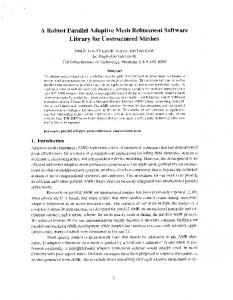
Since D = [0, 1] we consider dyadic grids of the form Vj = {xj,k ∈ [0, 1] : xj,k = k/2j , 0 ≤ k ≤ 2j },

Jmin ≤ j ≤ Jmax ,

(2)

where j denotes the resolution level, k the spatial location, and Jmin , Jmax ∈ Z+ 0 . We denote by Wj the set of grid points belonging to Vj+1 \ Vj . Therefore, Wj = {yj,k ∈ [0, 1] : yj,k = (2k + 1)/2j+1 , 0 ≤ k ≤ 2j − 1},

Jmin ≤ j ≤ Jmax − 1.

(3)

Hence, xj+1,k ∈ Vj+1 is given by ( xj+1,k =

xj,k/2 , if k is even, yj,(k−1)/2 , otherwise.

(4)

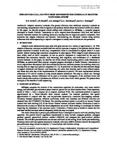
An example of a dyadic grid with Jmin = 0 and Jmax = 5 is shown in Figure 1.

V0

k=0

k=1

W0

k=0

W1

k=0

k=1

W2 k=0

W3 W4

k=3

k=0

k=7

k=0

k=15

Figure 1: Example of a dyadic grid. 3

With a slight abuse of notation we write Vj+1 = Vj ⊕ Wj ,

(5)

although Wj is not an orthogonal compliment of Vj in Vj+1 . The subspaces Vj are nested VJmin ⊂ VJmin +1 · · · ⊂ VJmax ,

(6)

with limJmax →∞ VJmax = D. On the contrary, the sequence of subspaces Wj satisfy Wj ∩ W` = ∅,

3.1

j 6= `.

(7)

Grid Adaptation

Assume we are given a nonuniform grid of the form Grid =

{xji ,ki : xji ,ki ∈ [0, 1], 0 ≤ ki ≤ 2ji , Jmin ≤ ji ≤ Jmax , for i = 0 . . . N, and xji ,ki < xji+1 ,ki+1 , for i = 0 . . . N − 1}.

(8)

For simplicity of notations, we denote u(x, t) evaluated at x = xj,k and t = n∆t by unj,k , where 0 ≤ k ≤ 2j , Jmin ≤ j ≤ Jmax , n ∈ Z+ 0 , and ∆t is the time step based on the Courant-FriedrichsLevy condition [42] for hyperbolic equations and the von Neumann condition [42] for all other evolution equations. For grid adaptation we first need a procedure for computing the function value at any point xinterp ∈ (0, 1) from the function values in U = {unj,k : xj,k ∈ Grid}, using an interpolating

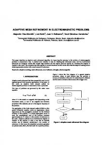
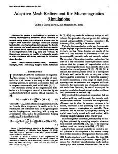
i+p ∈ Grid polynomial of degree p. To this end, the first step is to find the p+1 nearest points {xj` ,k` }`=i to xinterp , where 0 ≤ i ≤ N − p. By p + 1 nearest points here we mean one neighboring point on the left of xinterp , one neighboring point on the right of xinterp and the remaining p − 1 points are the points nearest to xinterp in the set Grid. In case two points are at the same distance, that is, if a point on the left and a point on the right are equidistant to xinterp , then we choose a point so as to equalize the number of points on both sides. For example, consider a grid at level j = 3 as shown in Figure 2. The set Grid consists of the solid circles. Let p = 3 and xinterp = x3,4 , shown by an empty square in Figure 2. The whole process involves three steps. Step a: We include in the set Xnear one neighboring point on the left (x3,2 ), shown by a left triangle and one neighboring point on the right (x3,5 ), shown by a right triangle in Figure 2. Step b: We add to the set Xnear the point x3,6 since the distance from xinterp to x3,0 is greater than the distance of xinterp to x3,6 . Step c: To choose the last point, we see that both points x3,0 and x3,8 are equidistant to xinterp . In this case, we choose x3,0 in order to equalize the number of points on both sides. Hence, our final set Xnear consists of points x3,0 , x3,2 , x3,5 , and x3,6 as shown in Figure 2. Suppose p is even and suppose we have already chosen p − 2 points based on the previous methodology, such that (p − 2)/2 points are on the left of xinterp and the remaining (p − 2)/2 points are on the right of xinterp . In case both points on the left and the right are equidistant to xinterp we choose either of these points as the last point. Note that this situation will not arise if p is odd. Once we have found the p + 1 nearest points, we construct an interpolating polynomial Lp (x) of order p passing through these p + 1 points. One may use Neville’s algorithm to construct the respective interpolating polynomials on the fly. The interpolating polynomials can also be constructed using high-resolution schemes such as by using the idea of ENO scheme [23, 40]. The only difference in that case would be that we would take one neighboring point on the left and one

4

Grid k=0

k=1

k=2

k=3

k=4

k=5

k=6

k=7

k=8

Step a: X near Step b: X near Step c: X near Figure 2: Demonstration of the procedure for finding the nearest points. neighboring point on the right of xinterp , and choose the remaining p − 1 points that give the least oscillatory polynomial. The algorithm described above for calculating the function value at xinterp from the function values in U , using an interpolating polynomial of degree p, is summarized in the following psuedocode: INTERPNEAREST(xinterp , Grid, U, p) 1 Xnear = {xj` ,k` }i+p `=i ; the p + 1 nearest points to xinterp in the set Grid; 2 Construct Lp (x) using the points in the set Xnear and the corresponding function values in U ; 3 Calculate Lp (xinterp ). The “top-down” approach of our algorithm allows us to add and remove points using the most updated information. Now suppose u(x, n∆t) is specified on a grid Gridold , with corresponding solution values Uold = {unj,k : xj,k ∈ Gridold }, (9) where Gridold can be either regular or irregular2 . Our aim is to find a new grid Gridnew , by adding or removing points from Gridold , reflecting local changes in the solution. To this end, we initialize an intermediate grid Gridint = VJmin . We then set j = Jmin and find the points belonging to the intersection of Wj and Gridold . To this end, let this intersection be Y = {yj,ki : yj,ki ∈ Wj ∩ Gridold , for i = 1, . . . , M }.

(10)

Now we find the interpolated function value u ˆj,k1 at point yj,k1 ∈ Y from the points in Gridint and their function values in the set Uint = {unj,k : unj,k ∈ Uold and xj,k ∈ Gridint } using the procedure INTERPNEAREST mentioned above. Next we find the interpolative error coefficient dj,k1 at the point yj,k1 . Definition 1. The interpolative error coefficient dj,k at any point yj,k ∈ Wj , where Jmin ≤ j ≤ Jmax − 1 and 0 ≤ k ≤ 2j − 1, is defined as dj,k = |u(yj,k , n∆t) − u ˆ(yj,k )|.

(11)

The interpolative error coefficient is a measure of the local smoothness of the function. If the value of dj,k is below the prescribed threshold ², then yj,k is rejected since the function value at this point can be reconstructed from the points in grid Gridint with an error no larger than ². A function with isolated singularities but is otherwise regular, will have most of the interpolative error 2

Typically, Gridold at time t = 0 is regular with Gridold = VJmax .

5

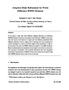
coefficients close to zero. This allows a compact approximation of the function without significant loss of accuracy. If the value of dj,k1 is above the prescribed threshold ², we add yj,k1 to the intermediate grid Gridint , along with N1 points on the left and N1 points on the right neighboring to the point yj,k1 in Wj . This step accounts for the possible displacement of any sharp features of the solution during the next time integration step. The value of N1 dictates the frequency of mesh adaptation and is provided by the user. At the same time, we add to Gridint 2N2 neighboring points at the next 2 level {yj+1,2k1 +` }N `=−N2 +1 . This step accounts for the possibility of the solution becoming steeper in this region and the value of N2 is chosen based on the problem. We also add the function values at all the newly added points to Uint . If the function value at any of the newly added points is not known, we interpolate the function value at that point from the points in Gridold and their function values in Uold using the procedure INTERPNEAREST. Next we move to point yj,k2 ∈ Y and repeat the whole process, and similarly for all yj,ki , i = 3, . . . , M . Once we have checked all the points in Y , we set j = j + 1, and repeat the above mentioned steps until j = Jmax − 1. This way we obtain the new nonuniform grid Gridnew . In this work we consider two choices for the threshold ². We can set either ² = ²ˆ or ² = ²ˆ/2j/2 , where ²ˆ > 0 is chosen based on the desired accuracy in the solution. The choice ² = ²ˆ implies that ² is the same for all Wj , whereas the choice ² = ²ˆ/2j/2 implies that ² changes with each level Wj . In this case ² becomes increasingly smaller as one goes from j = Jmin to j = Jmax − 1. This is to account for the reduction in the interpolation error with the decrease in the distance between the interpolating points. We use ² = ²ˆ/2j/2 for the case when the initial condition is not smooth and ² = ²ˆ for the case when the initial condition is smooth. A pseudocode for the above mentioned grid adaptation procedure is as follows: GRIDSELECTION(Gridold , Uold , Jmin , Jmax , VJmax , p, ², N1 , N2 ) 1 Gridint = VJmin ; 2 Uint = {unj,k : unj,k ∈ Uold and xj,k ∈ Gridint }; 3 for j = Jmin to Jmax − 1 4 Y = {yj,k : yj,k ∈ Wj ∩ Gridold }; 5 for every yj,k ∈ Y 6 u ˆ(yj,k ) = INTERPNEAREST(yj,k , Gridint , Uint , p); 7 dj,k = |u(yj,k , n∆t) − u ˆ(yj,k )|; 8 if dj,k > ² 1 9 Add points {yj,k+` }N `=−N1 to Gridint ; 2 10 Add points {yj+1,2k+` }N `=−N2 +1 to Gridint ; 11 Add the function values at all the newly added points to Uint ; 12 Empty Y ; 13 Gridnew = Gridint ; Unew = Uint . Next, we explain the proposed grid adaptation algorithm with the help of a simple toy example. Example 1 Consider a dyadic grid V4 and the function ( 1, x = x4,k , g(x) = 0, otherwise,

(12)

with k = 6, so that g denotes an impulse located at x = x4,6 = 0.375. Let Jmin = 0, Jmax = 4, p = 1, ² = 0.1, N1 = N2 = 1, and consider Gridold = VJmax . For this example the proposed grid adaptation algorithm is illustrated in Figure 3. 6

g k=0

k=6

k=16

Grid int = VJmin = V0 W0 Grid int W1 Grid int W2 W2 W3 Grid int W2 Grid int W3 W3 Grid int W3 W3 Grid int W3 Grid new

Figure 3: Demonstration of GRIDSELECTION procedure using Example 1.

7

In Figure 3, the solid circles show the points belonging to the intermediate grid Gridint and those belonging to Gridnew . The empty squares show the points that are being tested or have been tested for inclusion in Gridint . If the interpolative error coefficient at a point is greater than the prescribed threshold then we show that point by a solid square. The left and the right neighbors are shown by left and right triangles, respectively. For reference, all points at that particular level are shown by empty circles. First, we initialize Gridint with VJmin . Next, we check if the function value at the point y0,0 ∈ W0 can be interpolated from the nearest p + 1 = 2 points in Gridint , which in this case are the points x0,0 and x0,1 . Since for this example g(y0,0 ) can be interpolated from the points in Gridint , we do not include y0,0 in Gridint . Next, we consider the level W1 and check the point y1,0 . Since g(y1,0 ) can again be interpolated from the function values at points x0,0 , x0,1 ∈ Gridint , we do not include y1,0 in Gridint , and move on to the next point y1,1 . For the same reason as before, we do not include this point and the point y2,0 belonging to the next level W2 . Moving further to y2,1 , we find that g(y2,1 ) cannot be interpolated from the neighboring two points x0,0 , x0,1 ∈ Gridint . Hence, we include y2,1 in Gridint along with points y2,0 , y2,2 ∈ W2 and y3,2 , y3,3 ∈ W3 . Next, we check point y2,2 . The nearest points to y2,2 in Gridint are y3,3 and x0,1 . Since g(y2,2 ) can be interpolated from y3,3 and x0,1 , we do not include y2,2 in the grid. For the same reason, we do not include y2,3 . Now we move to the next level W3 and check points y3,0 and y3,1 . Since both these points can be interpolated from the existing points in Gridint we do not include these points in the grid. Subsequently we check y3,2 . Since g(y3,2 ) cannot be interpolated from the nearest two points y2,0 , y2,1 ∈ Gridint we include y3,2 along with points y3,1 and y3,3 (which in any case is already present in Gridint ) in Gridint . Moving on to the next point y3,3 , we see again that g(y3,3 ) cannot be interpolated from the nearest two points y2,1 , y2,2 ∈ Gridint . Hence, we include y3,3 along with y3,2 (which in any case is already present in Gridint ) and y3,4 in Gridint . The next point in W3 is y3,4 . Since g(y3,4 ) can be interpolated from the two nearest points y3,3 , y2,2 ∈ Gridint , we move on to the next point y3,5 . The nearest two points to y3,5 in Gridint are y2,2 , x0,1 , and since g(y3,5 ) can be interpolated from these two points, we do not include y3,5 in Gridint . For the same reason we do not add points y3,6 and y3,7 . The final adaptive grid Gridnew is shown by the solid circles in Figure 3. The adaptive grid generated using the previous algorithm depends on how we select points along the grid, that is, whether we move from left to right or from right to left across each level. It also depends on the location of the singularity. If the singularity is located in the middle, then it does not matter whether we move from left to right or from right to left. The result will be the same nonuniform grid. If on the other hand, the singularity is not in the middle, then the grid depends on the way in which we traverse across each level. To see this fact, we again consider Example 1, but this time with k = 1. Hence, the impulse is located at x = x4,1 . If we go from left to right then the adaptive grid consists of the points x4,0 , x4,1 , x4,3 , x4,5 , x4,16 . If we go from right to left then the grid consists of the points x4,0 , x4,1 , x4,3 , x4,16 . Now let k = 15, which implies that the impulse is located at x = x4,15 . If we go from left to right then the grid consists of the points x4,0 , x4,13 , x4,15 , x4,16 , and if we go from right to left then the grid consists of the points x4,0 , x4,11 , x4,13 , x4,15 , x4,16 . Note that in the proposed algorithm it is not mandatory to traverse across a level only from the leftmost point or from the rightmost point. We can instead start from any point at that level, each time resulting in a different grid. This suggests that by using a suitable probability distribution function to choose the order in which the points at each particular level are selected, one may be able to further optimize the grid. We will not elaborate on this observation in this paper.

8

3.2

The Traditional Grid Adaptation Approach

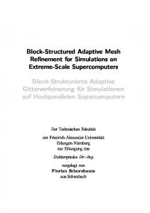
In this section, we briefly summarize the main idea underlying the traditional grid adaptation approach. For the details on the traditional grid adaptation approach the reader is referred to [3, 20, 21, 24]. Consider a set of dyadic grids Vj and Wj as described in equations (2) and (3) before. We explain pictorially, with the help of Example 1, how the traditional approach works (see Figure 4). The symbols used in Figure 4 are the same as those used in Figure 3 except for a new symbol (a triangle facing down), which is used to show the parents of points in Wj , that is, the points in Vj that are used for interpolating the function values at points in Wj . In the traditional approach, we first interpolate the function values at the points belonging to Wj from the corresponding points in Vj for j = 0, . . . , 3, respectively, as shown in Figure 4. Then we find the points which have interpolative error coefficients greater than the prescribed threshold ². We see that points y2,1 , y3,2 , y3,3 have interpolative error coefficients greater than the threshold (shown by solid squares) and add these points in the grid. Next, we add the points y2,0 , y2,2 neighboring to y2,1 in W2 (shown by level A) and the points y3,2 , y3,3 neighboring to y2,1 in W3 (shown by level B). Similarly, we add points y3,1 , y3,3 neighboring to y3,2 in W3 (shown by level C) and the points y3,2 , y3,4 neighboring to y3,3 in W3 (shown by level D). Finally, we include the parents of all the points added previously to the adaptive grid (shown by levels Ap , Bp , Cp and Dp ) resulting in the nonuniform grid Gridnew shown in Figure 4.

3.3

Comparison between the Traditional and the Proposed Approach

The proposed grid adaptation algorithm results, in general, in a fewer number of grid points when compared to the traditional approach. First, we explain why this is so and then we give several examples to demonstrate this fact. j In the traditional approach, one interpolates {g(yj,k )}2k=0 only from the function values at the points belonging to Vj for j = Jmin . . . Jmax − 1, and only then, one adds to the adaptive grid, N2 1 the points yj,k along with the points {yj,k+` }N `=−N1 and {yj+1,2k+` }`=−N2 +1 for all the pairs (j, k), such that dj,k > ². In the proposed method, we continuously keep on updating the adaptive grid instead. If the interpolative error coefficient at yj,k , where 0 ≤ k ≤ 2j − 1 and Jmin ≤ j ≤ Jmax − 1, is greater than the prescribed threshold, we add yj,k to the adaptive grid, and at the same time 1 we add to the adaptive grid the neighboring points at the same level {yj,k+` }N `=−N1 , as well as 2 the neighboring points at the next level {yj+1,2k+` }N `=−N2 +1 . We use these newly added points also for interpolating the remaining points at level Wj and the levels below it. In other words, j in the proposed approach, {g(yj,k )}2k=0 are interpolated from the function values at the points in Vj ⊕ Wj ⊕ Wj+1 for Jmin ≤ j ≤ Jmax − 2 and in Vj ⊕ Wj for j = Jmax − 1. Hence, by making use of the extra information from levels Wj and Wj+1 , which in any case will be added to the adaptive grid, we are able to reduce the number of grid points in the final grid. Moreover, in the traditional approach, when a point yj,k , where 0 ≤ k ≤ 2j − 1 and Jmin ≤ j ≤ Jmax − 1, is added to the grid then we also include its parents, which were used to predict the function value at that point. The parents are not needed for approximating g to the prescribed accuracy but are included just for calculating the interpolative error coefficient at the point yj,k during the next mesh adaptation. In the proposed algorithm, on the other hand, whenever a point is being checked for inclusion in the adaptive grid, we predict the function value at that point only from the points which already exist in the adaptive grid. Hence, if that point is inserted in the grid we do not need to add any extra points (i.e., its parents). This also saves us from keeping a separate track of the parents to distinguish them from the rest of the points as in the traditional approach. 9

g k=0

k=6

k=16

VJmin = V0 W0 V1 W1 V2 W2 A B V3 W3 C D

VJmin = V0 Ap A Bp B Cp C Dp D Grid new

Figure 4: Demonstration of traditional grid adaptation approach using Example 1.

10

Example 2 Consider a dyadic grid V4 and the function ( 1, x = x4,k , g(x) = 0, otherwise,

(13)

with an impulse located at x = k/24 , where 0 ≤ k ≤ 16. Let Jmin = 0, Jmax = 4, p = 1, ² = 0.1, and N1 = N2 = 1. Table 1 shows the number of grid points (Ng ) in the adaptive grid using both the traditional and the proposed methods for k = 0, . . . , 16. We found that when the impulse is located at either the left boundary (k = 0) or the right boundary (k = 16) or in the middle of the domain (k = 8) both the traditional approach and the proposed approach result in the same grid. For all other cases, the grids generated by both the algorithms are different and we see that the proposed algorithm results in a fewer number of grid points. For this example the proposed algorithm outperforms the traditional approach by up to 33%. k 0 1 2 3 4 5 6 7 8 9 10 11 12 13 14 15 16

Ng using Traditional Method 9 6 9 8 12 9 12 9 13 9 12 9 12 7 9 6 9

Ng using Proposed Method 9 5 7 6 11 6 9 6 13 6 9 6 11 5 7 4 9

Ratio 1 0.83 0.78 0.75 0.92 0.67 0.75 0.67 1 0.67 0.75 0.67 0.92 0.71 0.78 0.67 1

Table 1: Example 2. Traditional method vs proposed method. Example 3 Now consider another example with g(x) a step function, given by ( 1, 13 ≤ x ≤ 23 , g(x) = 0, otherwise.

(14)

For this example, we consider a grid with Jmin = 2 and Jmax = 10. The results for different thresholds using interpolating polynomials of degree p = 1 and p = 3 are summarized in Table 2. We consider N1 = N2 = 1. In this example we found that if the points are predicted using linear interpolation both the algorithms result in the same grids for different thresholds, whereas if the 11

p

²

1 1 3 3 3 3

0.3 0.1 0.05 0.01 0.001 0.0001

Ng using Traditional Method 51 51 89 89 89 89

Ng using Proposed Method 51 51 76 76 76 76

Ratio 1 1 0.85 0.85 0.85 0.85

Table 2: Example 3: Traditional method vs proposed method. points are predicted using cubic interpolation, the algorithms result in different grids, and the proposed algorithm always results in approximately 15% fewer number of points. Example 4 Next, we consider the function 2

g(x) = sin(2πx) + e−β(x−0.5) ,

(15)

which is smooth everywhere except for the peak at x = 0.5. Here β is a parameter that controls the width of the Gaussian. We let β = 20000. For this example we let Jmin = 2, Jmax = 10, p = 3, and N1 = N2 = 1. The results for different thresholds are summarized in Table 3. We observe once ² 10−2 10−3 10−4 10−5 10−6 10−7 10−8 10−9 10−10

Ng using Traditional Method 69 89 125 181 277 429 545 1005 1025

Ng using Proposed Method 49 79 116 150 185 304 530 957 1021

Ratio 0.71 0.89 0.93 0.83 0.67 0.71 0.97 0.95 0.99

Table 3: Example 4. Traditional method vs proposed method. again that the proposed algorithm outperforms the traditional approach by up to 33%. We are now ready to present the algorithm for solving the (IBVP) on an adaptive, nonuniform grid.

4

Numerical Solution of the IBVP for Evolution Equations

The numerical scheme for discretizing (IBVP) depends on f (uxx , ux , u, x). The proposed grid adaptation algorithm will work for many numerically stable discretization schemes for (IBVP). We use different schemes for different numerical examples discussed in this paper depending on the problem. Hence, in the next section we only describe the techniques we use for calculating the 12

spatial derivatives ux and uxx on the nonuniform grid and we state the numerical schemes in the examples themselves.

4.1

Calculation of the Spatial Derivatives

For calculating the derivative ux on the adaptive nonuniform grid Gridnew we extend the essentially nonoscillatory (ENO) [23, 40, 41] and weighted ENO (WENO) schemes [28, 29, 32, 37] to nonuniform grids. To this end, let the nonuniform grid be given as in (8). Now define D+ unji ,ki

=

unji+1 ,ki+1 − unji ,ki xji+1 ,ki+1 − xji ,ki

D− unji ,ki

,

=

unji ,ki − unji−1 ,ki−1 xji ,ki − xji−1 ,ki−1

.

(16)

n ± A third-order ENO approximation to (u± x )ji ,ki = ux (xji ,ki , n∆t) is given by one of the following expressions v1 7v2 11v3 n ((u± − + (17) x )ji ,ki )1 = 3 6 6 or v2 5v3 v4 n ((u± + + (18) x )ji ,ki )2 = − 6 6 3 or v3 5v4 v5 n + − , (19) ((u± x )ji ,ki )3 = 3 6 6 n − n − n − n where for calculating (u− x )ji ,ki , we use v1 = D uji−2 ,ki−2 , v2 = D uji−1 ,ki−1 , v3 = D uji ,ki , v4 = n + n D− unji+1 ,ki+1 , v5 = D− unji+2 ,ki+2 , and for calculating (u+ x )ji ,ki , we use v1 = D uji+2 ,ki+2 , v2 = D+ unji+1 ,ki+1 , v3 = D+ unji ,ki , v4 = D+ unji−1 ,ki−1 , v5 = D+ unji−2 ,ki−2 . The basic idea behind a thirdn ± n ± n order ENO scheme is to choose either ((u± x )ji ,ki )1 or ((ux )ji ,ki )2 or ((ux )ji ,ki )3 for approximating ± n (ux )ji ,ki by choosing the smoothest possible polynomial interpolation of u. n It is reminded that a WENO approximation of (u± x )ji ,ki is a convex combination of the approximations in equations (17), (18) and (19), that is,

n (u± x )ji ,ki =

3 X

n ω` ((u± x )ji ,ki )` ,

(20)

`=1

where 0 ≤ ω` ≤ 1 for ` = 1, 2, 3 and ω1 + ω2 + ω3 = 1. The weights for a fifth-order accuracy are given by [28, 37] α` ω` = , ` = 1, 2, 3, (21) α1 + α2 + α3 where α` =

α ¯` , (S` + δ)2

` = 1, 2, 3,

13 1 (v1 − 2v2 + v3 )2 + (v1 − 4v2 + 3v3 )2 , 12 4 1 13 S2 = (v2 − 2v3 + v4 )2 + (v2 − v4 )2 , 12 4 13 1 S3 = (v3 − 2v4 + v5 )2 + (3v3 − 4v4 + v5 )2 , 12 4 S1 =

13

(22) (23) (24) (25)

and α ¯ 1 = 0.1,

α ¯ 2 = 0.6,

α ¯ 3 = 0.3.

(26)

In (22) δ is used to prevent the denominator from becoming zero. In our computations, we have used δ = 10−6 . For calculating uxx , we extend the centered second difference scheme for the uniform mesh [42] to the nonuniform mesh (8) as follows µ n ¶ n uj −un un ,k j ,k j ,k −uj ,k 2 xni+1 i+1 −xni i − xni i −xni−1 i−1 ji+1 ,ki+1 ji ,ki ji ,ki ji−1 ,ki−1 (uxx )nji ,ki = . (27) n n xji+1 ,ki+1 − xji−1 ,ki−1 Now we are ready to give the algorithm for solving IBVP for evolution equations (1).

4.2

Solution of the IBVP for Evolution PDEs

Based on the problem and the desired accuracy we choose the minimum resolution level Jmin , the maximum resolution level Jmax , the threshold ², the order of the interpolating polynomial p and the parameters N1 , N2 required for the GRIDSELECTION procedure. The final time tf is assumed to be given. Jmax To solve (IBVP) on an adaptive grid, we first initialize Gridold = VJmax and Uold = {g(xJmax ,k )}2k=0 . Next, we find the new grid Gridnew and the function values at all the points in Gridnew , Unew = {unj,k : xj,k ∈ Gridnew }, using the GRIDSELECTION procedure. The new grid Gridnew is the grid on which we will propagate the solution from time t = 0 to time t = ∆tadapt , where ∆tadapt is the time after which the grid should be adapted again. It is calculated based on the approximate time the solution will take to move N1 grid points. Therefore, the value of N1 will dictate the frequency of mesh adaptation. The larger the N1 , the smaller the frequency of mesh adaptation will be, at the expense of a larger number of grid points in the adaptive grid. Hence, there is a trade-off between the frequency of mesh adaptation and the number of grid points. Next, we find the solution at time t + ∆t at all the points belonging to Gridnew , with values Unew = {un+1 j,k : xj,k ∈ Gridnew }, using any numerically stable scheme. This way we keep on propagating the solution on Gridnew until t < ∆tadapt . We then reassign the sets Gridold , Uold to Gridnew , Unew respectively, and find the new time at which the next mesh adaptation should take place tadapt = t + ∆tadapt . We keep on repeating the above mentioned steps until the final time tf is reached. A pseudocode of the above algorithm is as follows:

14

IBVP EE(g, tf , Jmin , Jmax , VJmax , p, ², N1 , N2 ) 1 t = 0, n = 0; Jmax 2 Gridold = VJmax ; Uold = {g(xJmax ,k )}2k=0 ; 3 tadapt = ∆tadapt ; 4 while (t ≤ tf ) do 5 [Gridnew , Unew ] = GRIDSELECTION(Gridold , Uold , Jmin , Jmax , VJmax , p, ², N1 , N2 ); 6 while t < tadapt do 7 find Unew = {un+1 j,k : xj,k ∈ Gridnew } using any numerically stable scheme; 8 t = t + ∆t; n = n + 1; 9 Empty Gridold , Uold ; 10 Gridold = Gridnew ; Uold = Unew ; 11 Empty Gridnew , Unew ; 12 tadapt = t + ∆tadapt ; 13 Gridnew = Gridold ; Unew = Uold .

5

Numerical Examples

In this section we present several examples to demonstrate the stability and robustness of our algorithm. These examples also validate the extension of ENO, WENO, and second difference schemes to the nonuniform grid and illustrate the algorithm’s ability to automatically capture and follow any existing or self-sharpenning features of the solution that develop in time. Example 5 Consider the linear advection equation ut + ux = 0,

(28)

u(0, t) = u(1, t),

(29)

with the periodic boundary condition

and initial condition

( g(x) =

1, 1/3 ≤ x ≤ 2/3, 0, otherwise.

(30)

The final time is tf = 0.5 s. We approximate ux by u− x using a third-order ENO scheme and use a third-order TVD RK scheme [40] for temporal integration. The numerical solution at the final time using a grid with Jmin = 4 and Jmax = 14 is shown in Figure 5(a). The other parameters used in the GRIDSELECTION procedure are p = 1, ² = 0.001/2j/2 , N1 = 2, and N2 = 1. The grid point distribution in terms of position and resolution level at t = 0.50024 s is shown in Figure 5(b). The regions where the solution is smooth are well represented by the coarse resolution levels; the higher resolution levels are needed only near the edges of the step function, thus illustrating the efficient data compression of the adaptive strategy proposed in this paper. Since the numerical scheme is dissipative, the sharp edges of the step function tend to smear out continuously. Hence, the grid adaptation algorithm is continuously adding points near the edges to maintain the desired accuracy. This can also be observed by looking at the time evolution of the number of grid points in Figure 5(c). We see that the number of grid points is constantly increasing, which again shows the efficiency of the proposed grid adaptation algorithm. A comparison of CPU times for the uniform

15

t= 0.50024 Points: 309 out of 16385 1.2

14 13

1 12 0.8

11 10

0.6 j

u(x)

Numerical Sol. Initial Condition 0.4

9 8 7

0.2

6 0 5 −0.2

0

0.2

0.4

0.6

0.8

4

1

0

0.2

0.4

0.6

0.8

1

x

x

(a) Solution u(x, 0.50024).

(b) Grid point distribution at t = 0.50024 s.

350

300

Ng

250

200

150

100

50

0

0.1

0.2

0.3

0.4

0.5

t

(c) Time evolution of the number of grid points.

Figure 5: Example 5. Parameters used in the simulation are Jmin = 4, Jmax = 14, p = 1, ² = 0.001/2j/2 , N1 = 2, and N2 = 1. and adaptive grids, along with the average number of points used for Jmax = 10, 11, 12, 13, 14 are summarized in Table 4. In the next two examples we consider the evolution equation (1) with f (uxx , ux , u, x) = f (ux , u, x).

(31)

We use the Lax-Friedrich’s (LF) scheme [14, 37, 38, 41] for discretizing f (ux , u, x) as follows µ + ¶ ux + u− 1 x LF − + − ˆ f (ux , u, x) = f (ux , ux , u, x) = f , u, x − αx (u+ (32) x − ux ), 2 2 where, αx = maxx |f1 (ux , u, x)|, ux ∈I

(33)

max where f1 is the partial derivative of f with respect to ux , I x = [umin x , ux ], and the minimum + and the maximum values of ux are identified by considering all the values of u− x and ux on the

16

Jmax 10 11 12 13 14

Uniform Mesh Ng in VJmax tcpu (s) 210 + 1 = 1025 0.2715 11 2 + 1 = 2049 1.4821 212 + 1 = 4097 5.6090 13 2 + 1 = 8193 22.2160 214 + 1 = 16385 85.6133

Adaptive Mesh Ng ave in Gridnew tcpu (s) Speed Up 135 0.0907 3.0 159 0.1914 7.7 188 0.4788 11.7 222 1.3575 16.4 264 4.1690 20.5

Table 4: Example 5. Computational times for uniform vs. adaptive mesh. nonuniform grid. Example 6 We again consider the linear advection equation ut − ux = 0,

(34)

u(0, t) = u(1, t),

(35)

with periodic boundary condition and initial condition

2

g(x) = sin(2πx) + e−β(x−1/2) .

(36)

As mentioned earlier the initial function is mostly smooth with a peak located at x = 0.5. Here we again consider β = 20000. The final time is tf = 0.3 s. Since we are solving a linear advection equation, we may approximate ux by u+ x as we did in the previous example where we approximated ux by u− . We use an LF scheme to check the accuracy of the scheme on the resulting nonuniform x − grid since the exact solution of this problem is known. We approximate the derivatives u+ x , ux in the LF discretization using a WENO scheme and use a third-order TVD RK scheme for temporal integration. The numerical results using a grid with Jmin = 5 and Jmax = 14 are shown in Figure 6. The other parameters used in the GRIDSELECTION procedure are p = 3, ² = 0.02/2j/2 , and N1 = N2 = 2. As can be seen from Figure 6, the proposed grid adaptation algorithm performed well with the LF scheme combined with a third-order TVD RK scheme. The grid point distribution (Figure 6(b)) again validates the efficiency of the proposed algorithm. A comparison of CPU times for the uniform and adaptive grids, along with the average number of points used for Jmax = 10, 11, 12, 13, 14 are summarized in Table 5. We see a major speed up in the computational time compared to the uniform mesh, and the speed-up factors increase significantly with mesh refinement at an approximate rate of two. There is a trade-off between

Jmax 9 10 11 12

Uniform Mesh Ng in VJmax tcpu (s) 9 2 + 1 = 513 8.0605 210 + 1 = 1025 43.3547 211 + 1 = 2049 190.4138 212 + 1 = 4097 747.6864

Adaptive Mesh Ng ave in Gridnew tcpu (s) 70 1.2635 87 3.9434 103 8.0187 105 14.6014

Speed Up 6.4 11.0 23.7 51.2

Table 5: Example 6. Computational times for uniform vs. adaptive mesh. accuracy and speed up of computations. We solved this problem again for Jmax = 12 using the 17

t= 0.3 Points: 109 out of 4097 12 1 0.8

11

0.6 10 0.4 9 j

u(x)

0.2 0

8 −0.2 −0.4

7

−0.6 6 Numerical Sol. Initial Condition

−0.8 −1

0

0.2

0.4

0.6

0.8

5

1

0

0.2

0.4

0.6

0.8

1

x

x

(a) Solution u(x, 0.3).

(b) Grid point distribution at time t = 0.3 s.

125 120 115 110

Ng

105 100 95 90 85 80

0

0.05

0.1

0.15

0.2

0.25

0.3

0.35

t

(c) Time evolution of the number of grid points.

Figure 6: Example 6. Parameters used in the simulation are Jmin = 5, Jmax = 12, p = 3, ² = 0.02/2j/2 , and N1 = N2 = 2. same parameters as before, but this time with ² = 0.01/2j/2 and ² = 0.005/2j/2 . The numerical solution at the final time for both thresholds are shown in Figure 7. From Figure 7 we see that as we decrease the threshold, the dissipation in the height of the peak is decreasing at the cost of a greater CPU time, 22.1503 s for ² = 0.01/2j/2 and 29.0653 s for ² = 0.005/2j/2 . However, it should be noted that the CPU time for both the cases is still significantly less compared to the CPU time for the case of a uniform mesh. Example 7 In this example we solve the inviscid Burger’s equation ut + uux = 0.

(37)

Burger’s equation is similar to the linear advection equations (28) and (34), except from the fact that the convective term is nonlinear, thus allowing discontinuous solutions to develop in time even if the initial condition is smooth. We use the same smooth initial condition and the Dirichlet

18

boundary condition as in [3], that is, g(x) = sin(2πx) +

1 sin(πx), 2

(38)

u(0, t) = u(1, t) = 0,

(39)

to check the ability of the proposed algorithm to capture the shock. The solution is a wave that develops a very steep gradient and subsequently moves towards x = 1. Because of the zero boundary values, the wave amplitude diminishes with increasing time. + We use a WENO scheme for calculating the derivatives u− x , ux in the LF discretization and we use a third-order TVD RK method for temporal integration. The numerical solutions at different times t = 0 s, t = 0.158 s, t = 0.5 s and t = 1 s using a grid with Jmin = 4 and Jmax = 12 are shown in Figure 8(a). The other parameters used in the GRIDSELECTION procedure are p = 3, ² = 0.0005, N1 = 2, and N2 = 1. Figure 8 also shows the grid point distribution in the adaptive mesh at times t = 0 s, t = 0.14 s, t = 0.158 s and t = 1 s. We see that as the shock continues to develop the algorithm adds points at the finer levels of resolution in the region where the shock is developing, and removes points from the regions where the solution is getting smoother and smoother. Similar conclusions can be drawn by looking at the time evolution of the number of grid points (Figure 8(f)). We see in the Figure 8(f) that the number of grid points is increasing as the shock continues to develop, and once the discontinuity appears in the solution the number of grid points starts to decrease since the solution is getting smoother in most of the remaining region. Once the solution is smooth everywhere except for the region of the shock the number of grid points is pretty much steady oscillating about a mean value of 68. This clearly shows that the proposed strategy uses only the grid points that are actually necessary to attain a given precision, and the algorithm is able to add and remove points when and where is needed. A comparison of CPU times for the uniform and adaptive grids, along with the average number of points used for different Jmax = 8, 9, 10, 11, 12 are summarized in Table 6. We observe a major speed up in the computational time compared to the uniform mesh, and the speed-up factors are again increasing at an approximate rate of two with mesh refinement showing the efficiency and good performance of our algorithm.

Jmax 8 9 10 11 12

Uniform Mesh Ng in VJmax tcpu (s) 8 2 + 1 = 257 2.5474 29 + 1 = 513 18.1617 210 + 1 = 1025 137.6709 211 + 1 = 2049 1142.5316 212 + 1 = 4097 9352.2561

Adaptive Mesh Ng ave in Gridnew tcpu (s) 49 0.5319 55 2.1699 59 9.1435 65 43.8749 69 188.9315

Speed Up 4.8 8.4 15.1 26.0 49.5

Table 6: Example 7. Computational times for uniform vs. adaptive mesh. Example 8 Consider the scalar reaction-diffusion problem from combustion theory [1, 31] Reδ (1 + a − u)e−δ/u = 0, aδ ux (0, t) = 0, u(1, t) = 1,

ut − uxx −

19

(40) (41)

u(x, 0) = 1.

(42)

The solution u represents the temperature of a reactant in a chemical system, a is the heat release, δ is the activation energy, and R is the reaction rate. For small times the temperature gradually increases from unity with a “hot spot” forming at x = 0. At a finite time, ignition occurs, and the temperature at x = 0 jumps rapidly from near unity to near 1 + a. A flame front then forms and propagates towards x = 1 with speed proportional to eaδ/2(1+a) . In real problems, a is about unity and δ is large, thus the flame front moves exponentially fast after ignition. We use the same problem parameters as in [1] namely, a = 1 and R = 5. We use δ = 30 as in [26, 39] since the flame layer in this case is much thinner, and higher mesh adaptation is required. We use (27) to discretize uxx and use a second-order TVD RK scheme [40] for temporal integration. To illustrate how we apply Neumann boundary condition on a nonuniform grid we again consider the grid of the form (8). To apply the Neumann boundary condition ux (0, t) = 0 we introduce a fictitious node xj−1 ,k−1 = −xj1 ,k1 . We approximate the boundary condition by3 (ux )nj0 ,0 =

unj1 ,k1 − unj−1 ,k−1 xj1 ,k1 − xj−1 ,k−1

= 0,

(43)

which implies unj−1 ,k−1 = unj1 ,k1 . Hence, at the boundary x = 0, equation (27) reduces to µ n ¶ n un u −un j ,0 −uj ,k 2 xjn1 ,k1 −xnj0 ,0 − xn0 −xn−1 −1 2(unj1 ,k1 − unj0 ,0 ) j0 ,0 j0 ,0 j1 ,k1 j−1 ,k−1 = (uxx )nj0 ,0 = . xnj1 ,k1 − xnj−1 ,k−1 (xnj1 ,k1 − xnj0 ,0 )2

(44)

(45)

The numerical solutions at times t = 0 s, t = 0.24 s, t = 0.2403 s, t = 0.24035 s, t = 0.241 s and t = 0.244 s using a grid with Jmin = 4 and Jmax = 10 are shown in Figure 9(a). The other parameters used in the GRIDSELECTION procedure are p = 3, ² = 0.001, N1 = 2, and N2 = 1. One of the main challenges of this problem is the fact that one needs to use a very small time step to capture the transition layer during the time of ignition. This is achieved automatically by the proposed algorithm since the proposed algorithm is adaptive both in time and space. As the mesh gets refined, ∆t in the procedure IBVP EE also decreases. In Figure 9(f) we show the time evolution of grid points starting at t = 0.23 s since the number of points for t ≤ 0.23 s remains constant. We see from Figure 9(f) that for time t < 0.239 s the proposed algorithm found the solution at grid V4 and efficiently added points at finer levels starting at t = 0.239 s. As the points from finer grid levels are being added, the algorithm automatically decreases the time step and is able to accurately capture the transition layer during the time of ignition. A comparison of CPU times for the uniform and adaptive grids, along with the average number of points used for Jmax = 8, 9, 10 are summarized in Table 7. We see again that speed-up factors are increasing with mesh refinement.

6

Conclusions

In this paper, we have proposed a novel grid adaptation algorithm, which is shown to outperform the traditional grid adaptation approach. Specifically, we showed that the proposed approach results 3

Note that k0 = 0.

20

Jmax 8 9 10

Uniform Mesh Ng in VJmax tcpu (s) 28 + 1 = 257 11.3496 29 + 1 = 513 86.0208 210 + 1 = 1025 646.5237

Adaptive Mesh Ng ave in Gridnew tcpu (s) 39 0.9141 51 3.9216 59 18.4145

Speed Up 12.4 21.94 35.1

Table 7: Example 8. Computational times for uniform vs. adaptive mesh. in fewer grid points in the grid compared to the traditional approach. For the examples considered here, we observed savings of up to 33% in terms of the number of grid points. We have solved the initial-boundary value problem for evolution equations in a computationally efficient manner using the proposed grid adaptation algorithm. The proposed algorithm is adaptive both in space and time. Moreover, the frequency of mesh adaptation is dynamically adjusted in order to optimize the algorithm even further. Several examples have demonstrated the stability and robustness of the proposed algorithm. The grid was able to adapt dynamically to any existing or emerging irregularities in the solution, and the grid point distribution (in terms of position and resolution level) is evident of this fact. In all examples considered, the algorithm was able to automatically allocate more grid points to the region where the solution exhibits sharp features and fewer points to the region where the solution is smooth, thereby reducing the computational time as well as the memory usage dramatically, while maintaining an accuracy equivalent to one obtained using a fine uniform mesh.

References [1] S. Adjerid and J.E. Flahery. A moving finite element method with error estimation and refinement for one-dimensional time dependent partial differential equations. SIAM Journal on Numerical Analysis, 23:778–795, 1986. [2] S. Adjerid and J.E. Flahery. A moving mesh finite element method with local refinement for parabolic partial differential equations. Computer Methods in Applied Mechanics and Engineering, 56:3–26, 1986. [3] M.A. Alves, P. Cruz, A. Mendes, F.D. Magalh˜aes, F.T. Pinho, and P.J. Oliveira. Adaptive multiresolution approach for solution of hyperbolic PDEs. Computer Methods in Applied Mechanics and Engineering, 191:3909–3928, 2002. [4] D.C. Arney and J.E. Flahery. A two-dimensional mesh moving technique for time dependent partial differential equations. Journal of Computational Physics, 67:124–144, 1986. [5] I. Babuˇska, J. Chandra, and J.E. Flaherty, editors. Adaptive Computational Methods for Partial Differential Equations. SIAM, Philadelphia, 1983. [6] M.J. Baines. Moving Finite Elements. Oxford University Press, New York, 1994. [7] M.J. Baines and A.J. Wathen. Moving finite element methods for evolutionary problems. I. Theory. Journal of Computational Physics, 79:245–269, 1988. [8] J. Bell, M.J. Berger, J. Saltzman, and M. Welcome. Three-dimensional adaptive mesh refinement for hyperbolic conservation laws. SIAM Journal on Scientific Computing, 15:127–138, 1994. 21

[9] M.J. Berger and P. Colella. Local adaptive mesh refinement for shock hydrodynamics. Journal of Computational Physics, 82:64–84, 1989. [10] M.J. Berger and R.J. Leveque. Adaptive mesh refinement using wave-propagation algorithms for hyperbolic systems. SIAM Journal on Numerical Analysis, 35:2298–2316, 1998. [11] M.J. Berger and J. Oliger. Adaptive mesh refinement for hyperbolic partial differential equations. Journal of Computational Physics, 53:484–512, 1984. [12] S. Bertoluzza. Adaptive wavelet collocation method for the solution of Burger’s equation. Transport Theory and Statistical Physics, 25:339–352, 1996. [13] N.N. Carlson and K. Miller. Design and application of a gradient weighted moving finite element code I: In one dimension. SIAM Journal on Scientific Computing, 19:728–765, 1998. [14] M. Crandall and P.L. Lions. Two approximations of solutions of Hamilton-Jacobi equations. Math. Comput., 43:1–19, 1984. [15] G. Deslauriers and S. Dubuc. Symmetric iterative interpolation processes. Constructive Approximation, 5:49–68, 1989. [16] D. L. Donoho. Interpolating wavelet transforms. Technical report, Department of Statistics, Stanford University, Stanford, CA, 1992. [17] E.A. Dorfi and L.O’c. Drury. Simple adaptive grids for 1-d initial value problems. Journal of Computational Physics, 69:175–195, 1987. [18] P.H. Gaskell and A.K.C. Lau. Curvature compensated convective transport: SMART, a new boundedness preserving transport algorithm. International Journal for Numerical Methods in Fluids, 8:617–641, 1988. [19] A. Harten. High resolution schemes for hyperbolic conservation laws. Journal of Computational Physics, 49:357–393, 1983. [20] A. Harten. Adaptive multiresolution schemes for shock computations. Journal of Computational Physics, 115:319–338, 1994. [21] A. Harten. Multiresolution algorithms for the numerical solution of hyperbolic conservation laws. Comm. Pure Appl. Math., 48:1305–1342, 1995. [22] A. Harten. Multiresolution representation of data: A general framework. SIAM Journal on Numerical Analysis, 33(3):1205–1256, 1996. [23] A. Harten, B. Enquist, S. Osher, and S. Chakravarthy. Uniformly high-order accurate essentially non-oscillatory schemes III. Journal of Computational Physics, 71:231–303, 1987. [24] M. Holmstrom. Solving hyperbolic PDEs using interpolating wavelets. SIAM Journal on Scientific Computing, 21, 1999. [25] M. Holmstrom and J. Walden. Adaptive wavelet methods for hyperbolic PDEs. Journal of Scientific Computing, 13(1):19–49, 1998. [26] W. Huang, Y. Ren, and R.D. Russell. Moving mesh methods based on moving mesh partial differential equations. Journal of Computational Physics, 113:279–290, 1994. 22

[27] L. Jameson. A wavelet-optimized, very high order adaptive grid and order numerical method. SIAM Journal on Scientific Computing, 19:1980–2013, 1998. [28] G.S. Jiang and D. Peng. Weighted ENO schemes for Hamilton-Jacobi equations. SIAM Journal on Scientific Computing, 21(6):2126–2143, 2000. [29] G.S. Jiang and C.W. Shu. Efficient implementation of weighted ENO schemes. Journal of Computational Physics, 126(1):202–228, 1996. [30] I.W. Johnson, A.J. Wathen, and M.J. Wathen. Moving finite element methods for evolutionary problems. II. Applications. Journal of Computational Physics, 79:270–297, 1988. [31] A.K. Kapila. Asymptotic treatment of chemically reacting systems. Pitman Advanced Publishing Program, Boston, 1983. [32] X.D. Liu, S. Osher, and T. Chan. Weighted essentially non-oscillatory schemes. Journal of Computational Physics, 115(1):200–212, 1994. [33] S. G. Mallat. Multiresolution approximations and wavelet orthonormal bases of L2 (R). In Transactions of the American Mathematical Society, volume 315, pages 69–87, 1989. [34] S.G. Mallat. A theory for multiresolution signal decomposition: The wavelet representation. IEEE Transactions on Pattern Analysis and Machine Intellegence, 2(7):674–693, 1989. [35] K. Miller. Moving finite elements II. SIAM Journal on Numerical Analysis, 18:1033–1057, 1981. [36] K. Miller and R.N. Miller. Moving finite elements I. SIAM Journal on Numerical Analysis, 18:1019–1032, 1981. [37] S. Osher and R.P. Fedkiw. Level Set Methods and Dynamic Implicit Surfaces. Springer, New York, 2003. [38] S. Osher and C.W. Shu. High order essentially non-oscillatory schemes for Hamilton-Jacobi equations. SIAM Journal of Numerical Analysis, 28:902–921, 1991. [39] L.R. Petzold. Observations on an adaptive moving grid method for one-dimensional systems for partial differential equations. Applied Numerical Mathematics, 3:347–360, 1987. [40] C.W. Shu and S. Osher. Efficient implementation of essentially non-oscillatory shock capturing schemes. Journal of Computational Physics, 77:439–471, 1988. [41] C.W. Shu and S. Osher. Efficient implementation of essentially non-oscillatory shock capturing schemes II. Journal of Computational Physics, 83:32–78, 1989. [42] J.W. Thomas. Numerical Partial Differential Equations. Springer, NY, 1995. [43] J.F. Thompson. A survey of dynamically-adaptive grids in the numerical solution of partial differential equations. Applied Numerical Mathematics, 1:3–27, 1985. [44] O.V. Vasilyev. Solving multi-dimensional evolution problems with localized structures using second generation wavelets. International Journal of Computational Fluid Dynamics, 17(2):151–168, 2003. 23

[45] O.V. Vasilyev and C. Bowman. Second-generation wavelet collocatioin method for the solution of partial differential equations. Journal of Computational Physics, 165:660–693, 2000. [46] J. Wald´en. Filter bank methods for hyperbolic PDEs. Journal of Numerical Analysis, 36:1183– 1233, 1999.

24

t= 0.3 Points: 131 out of 4097 12 1 0.8

11

0.6 10 0.4 9 j

u(x)

0.2 0

8 −0.2 −0.4

7

−0.6 6 Numerical Sol. Initial Condition

−0.8 −1

0

0.2

0.4

0.6

0.8

5

1

0

0.2

0.4

0.6

0.8

1

x

x

(a) Solution u(x, 0.3) for ² = 0.01/2j/2 .

(b) Grid point distribution at time t = 0.3 s for ² = 0.01/2j/2 .

t= 0.3 Points: 167 out of 4097 12 1 0.8

11

0.6 10 0.4 9 j

u(x)

0.2 0

8 −0.2 −0.4

7

−0.6 6 Numerical Sol. Initial Condition

−0.8 −1

0

0.2

0.4

0.6

0.8

5

1

0

0.2

0.4

x

0.6

0.8

1

x

(c) Solution u(x, 0.3) for ² = 0.005/2j/2 .

(d) Grid point distribution at time t = 0.3 s for ² = 0.005/2j/2 .

160

190

150

180 170

140

160 Ng

N

g

130 150

120 140 110

130

100

90

120

0

0.05

0.1

0.15

0.2

0.25

0.3

110

0.35

t

0

0.05

0.1

0.15

0.2

0.25

0.3

0.35

t

(e) Time evolution of the number of grid points for ² = (f) Time evolution of the number of grid points for ² = 0.01/2j/2 . 0.005/2j/2 .

Figure 7: Example 6. Parameters used in the simulation are Jmin = 5, Jmax = 12, p = 3, and N1 = N2 = 2. 25

1.6

12 t=0.0005

t=0.158 11

1.2 t=0.5 10 0.8

u(x)

t=1

9

j

0.4

8 7

0 6 −0.4 5 −0.8

0

0.2

0.4

0.6

0.8

4

1

0

0.2

0.4

x

12

12

11

11

10

10

9

9

8

8

7

7

6

6

5

5

0

0.2

0.4

0.6

0.8

4

1

0

0.2

0.4

x

11

100

10

90

9

80 Ng

j

110

8

60

6

50

5

40

0.4

0.8

1

70

7

0.2

0.6

(d) Grid point distribution at t = 0.158 s.

12

0

1

x

(c) Grid point distribution at t = 0.14 s.

4

0.8

(b) Grid point distribution at t = 0.0005 s.

j

j

(a) Solution u(x, t).

4

0.6 x

0.6

0.8

30

1

x

0

0.2

0.4

0.6

0.8

1

t

(e) Grid point distribution at t = 1 s.

(f) Time evolution of the number of grid points.

Figure 8: Example 7. Parameters used in the simulation are Jmin = 4, Jmax = 12, p = 3, ² = 0.0005, N1 = 2, and N2 = 1.

26

10 2 t=0.24035 9

t=0.241 1.8 t=0.244

8 t=0.2403 j

u(x)

1.6

7

1.4 6

t=0.24

1.2

5

1 t=0.0004 0.8

0

0.2

0.4

0.6

0.8

4

1

0

0.2

0.4

x

10

10

9

9

8

8

7

7

6

6

5

5

0

0.2

0.4

0.6

0.8

4

1

0

0.2

0.4

x

9

60

8

50

Ng

j

70

7

30

5

20

0.4

0.8

1

40

6

0.2

0.6

(d) Grid point distribution at t = 0.24035 s.

10

0

1

x

(c) Grid point distribution at t = 0.2403 s.

4

0.8

(b) Grid point distribution at t = 0.24 s.

j

j

(a) Solution u(x, t).

4

0.6 x

0.6

0.8

10 0.23

1

x

0.235

0.24

0.245

t

(e) Grid point distribution at t = 0.244 s.

(f) Time evolution of the number of grid points.

Figure 9: Example 8. Parameters used in the simulation are Jmin = 4, Jmax = 10, p = 3, ² = 0.001, N1 = 2, and N2 = 1.

27