Multiresolution Feature Detection in Adaptive Mesh Refinement with

Multiresolution Feature Detection in Adaptive Mesh Refinement with High-Order Shock- and Interface-Capturing Scheme Man Long Wong∗ Department of Aeronautics and Astronautics, Stanford University, Stanford, CA 94305, USA

Sanjiva K. Lele† Department of Aeronautics and Astronautics and Department of Mechanical Engineering, Stanford University, Stanford, CA 94305, USA A multiresolution wavelet detector is used as an extension of a second order derivative gradient detector in the adaptive mesh refinement (AMR) algorithm for identifying regions containing features of interest in single-species and multi-species compressible flows. The AMR algorithm is also successfully combined with the high order accurate and localized dissipative weighted compact nonlinear scheme1 (WCNS) for shock- and interface-capturing. Through different test problems, it is found that the multiresolution detector can capture discontinuities as well as the gradient sensor and has better performance over the latter sensor in identifying vortical features. Furthermore, by adding an additional constraint on the local regularity that is measured from wavelet coefficients at different scale levels, a significant number of redundant refined cells can be reduced with only a minimal effect on the accuracy of the solutions.

I.

Introduction

In recent years, AMR methods have become popular in the computational fluid dynamics (CFD) community due to its capability in capturing features in multi-scale physical problems with a considerable amount of savings in computational cost. These methods are commonly used in applications that involve highly compressible flows or multi-species mixing because of the localization of features of interest in these problems. For instance, in the regime of highly compressible flows, features such as shock waves or shocklets often appear only in confined regions and in the mixing of multi-fluids, one may require fine-scale resolution only in the regions of active mixing. Uniform discretization of computational domain is computationally inefficient when the flow features in some regions can be captured on a coarser mesh. AMR provides a way that can resolve those dynamically evolving features of interest by only adaptively refining a small portion of the computational domain. To achieve good adaptation of mesh refinement to the solution, a local error detector is critical. Berger and Colella2 suggested to estimate the local error for refinement with Richardson extrapolation which can estimate the local truncation error by comparing solutions on different grid resolutions. Despite its high accuracy in estimating error, it requires a large amount of computational resources because of extra time integration. The more computational efficient feature-based gradient detectors can be used in many applications to reduce cost. Although gradient detectors are robust in capturing sharp features such as shocks and contact discontinuities, it may be insufficient in sensing less local features such as vortices. In this paper, we tested two multiresolution wavelet detectors as an extension of a second order derivative gradient detector, in which one of these includes an additional constraint on the estimated local regularity in tagging cells for refinement. ∗ PhD.

Candidate, Department of Aeronautics and Astronautics, Stanford University, Stanford, CA 94305, USA Department of Aeronautics and Astronautics and Department of Mechanical Engineering, Stanford University, Stanford, CA 94305, USA, AIAA Associate Fellow † Professor,

1 of 26 American Institute of Aeronautics and Astronautics

Traditionally AMR is used with first/second order accurate finite difference/finite volume schemes. The low order schemes, while robust, are inefficient for obtaining high resolution solutions for flow problems that involve interactions between turbulence, shocks and material interfaces. As a results, there has been a growing interest in combining AMR algorithm with different high order accurate numerical methods. Li and Hyman3 were the first to combine the AMR method with high order finite difference weighted essentially non-oscillatory (WENO) scheme. Later, Baeza and Mulet4 also combined the AMR method with WENO scheme to simulate one- and two-dimensional shock-bubble interaction problems. Since it is well-known that traditional WENO schemes are too dissipative for high wavenumber features, Pantano et al.5 applied the AMR method on an improved low-numerical dissipation hybrid central finite difference/WENO scheme for large eddy simulation (LES) of shock- and discontinuity-containing turbulent flows. In this work, we combine the high order accurate hybrid weighted localized dissipative WCNS1 with the AMR algorithm to capture shock waves and contact discontinuities, and compare the performance of sensing multi-scale features between the gradient and multiresolution error detectors in various multi-dimensional test problems.

II.

Adaptive Mesh Refinement

An overview of the AMR algorithm is given in this section. The AMR algorithm in this work follows the one developed by Berger et al.,2 which was first developed specifically for hyperbolic equations. In a twodimensional space, the scalar hyperbolic equation for the dependent variable u can be written in the following form: ∂u ∂f (u) ∂g(u) + + =0 (1) ∂t ∂x ∂y where f (u) and g(u) are the fluxes in the x and y directions respectively. Berger’s AMR method assumes that the numerical scheme solves the hyperbolic equation in the explicit and conservative finite difference/volume form. This means after semi-discretization, the two-dimensional equation at a grid point (xi , yj ) with uniform grid spacings ∆x and ∆y is required to be in the following form: ˜ i,j+ 1 − G ˜ i,j− 1 F˜i+ 12 ,j − F˜i− 21 ,j G ∂ui,j 2 2 + + =0 ∂t ∆x ∆y

(2)

˜ i,j+ 1 can be interpreted as the fluxes at the cell edges in the x and y directions rewhere F˜i+ 12 ,j and G 2 specitively. A.

Hierarchical grid

Berger et al.2 ’s AMR algorithm is based on nested Cartesian grid patches. It requires a uniform rectangular root grid that discretizes the whole spatial domain. On top of the root grid, there is a hierarchy of sequentially nested grid patches. The grid patches are ordered into different levels l = 0, ..., lmax , where level 0 is the coarsest root level and lmax is the finest level. There may be more than one grid patch at each level but all grid patches Gl,k on the same level l must have the same mesh spacing ∆xl . Following Berger’s terminology,2 Gl is defined as the union of all grids at level l: [ Gl = Gl,k (3) k

As a results, the root grid is denoted by G0 . The grid patches are required to be properly nested such that a fine grid patch starts and ends at the corners of cells in the next coarser grid patch, and there must be a level l − 1 grid separating level l and level l − 2 grids. The mesh spacings between two consecutive grid levels l − 1 and l are related by a constant refinement ratio rl : rl =

∆xl−1 ∆xl

(4)

The refinement ratios between different consecutive grid levels can be different. In curent work, constant refinement ratio is used in the grid hierarchy.


B.

Grid refinement process

The grid refinement process is composed of a series of steps. Given a level of grids Gl , a detection procedure is first carried out to tag cells in Gl that need refinement. Berger2 proposed to use the Richardson extrapolation to estimate the local error for refinement. However, Richardardson extrapolation is expensive since it requires extra time integration of the solutions. In this paper, the less expensive gradient and multiresolution featurebased detectors are used and their performances of estimating local error are compared extensively through various test cases. The details and implementations of the detectors are discussed in another section. After regions of refinement interest are identified, buffer zones are added to prevent the features of interest to leave the refined regions during time integration. In this work, buffer zones of one cell width are used in all simulations. Cells that are tagged for refinement are then clustered into new Cartesian patches at one higher level. After new grid patches at finer level are produced, they are filled with initial conditions for time advancement. The initial conditions can be prepared by spatial interpolation from the solutions of coarser parent grids or using existing fine grid solutions. The linear spatial interpolation is adopted for projecting solutions from coarse grids to fine grids in this work. C.

Time refinement and integration

After the initial conditions on the new finer grids are initialized, the grids are advanced until regridding is necessary. For numerical stability reason, grids are not only refined in space but also in time such that ratio between time step ∆tl and grid spacing ∆xl is constant among all levels: ∆tl−1 ∆t0 ∆tl = = ... = =λ ∆xl ∆xl−1 ∆x0

(5)

where the constant λ can be determined from the CFL condition on the root grid solution. During the fine grid time integration, Dirichlet boundary conditions are used. The Dirichlet boundary conditions can be applied by using ghost cells in which their values are interpolated from solutions of the parent grids at different time levels. Linear temporal interpolation method is used in this work to obtain values of ghost cells from two consecutive time steps. During the time integration, grids at even finer levels are produced when regions of refinement interest are identified and the current level is not the highest level. The grid advancement at finer and finer levels forms a recursive algorithm. D.

Grid coarsening

With multiple grid levels and multiple grid patches at each level, we need to ensure consistency among solutions. Given coarser level of grids Gl and finer level of grids Gl+1 , the grids at coarser level are first advanced to t + ∆tl . After that, the ghost cells of the finer level grids at time levels t + k∆tl+1 , where k = 0, ..., rl+1 − 1, are interpolated from the solutions of coarser level grids at t and t + ∆tl . The solutions of finer level grids are then advanced to t + ∆tl . At this moment, the solutions of any cells in the coarser level grid has to be corrected if (i) the cell is covered by cells at finer level or (ii) the cell touches a finer grid interface even though it is not covered by any finer cells. The grid updating procedures for the two cases are described in the next two subsections. 1.

Coarse level cell covered by finer level cells

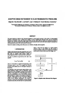
If cells are covered by finer level cells, the values of the coarser level cells are overwritten by the conservative average of the finer level cells. The cell (i, j) in Figure 1 is used as an example: uli,j ← 2.

1 2 rl+1

rl+1 −1 rl+1 −1

X

X

m=0

n=0

ul+1 ii+m,jj+n

(6)

Coarse level cell adjacent to a finer level grid but itself is not covered by any higher level cells

For any cells which are not covered by finer level cells but have cell edges connecting to finer grids, the fluxes across the coarse/fine cell boundaries are also adjusted. Otherwise, the finite difference scheme will not be conservative. The correction of flux at the vertical cell edge between finer level cells (ii + rl+1 − 1, jj + m), 3 of 26 American Institute of Aeronautics and Astronautics

where m = 0, ..., rl+1 − 1, and coarser level cell (i + 1, j) in Figure 1 is used as an example. After the time l+1 marching of grid Gl , we can initialize the flux correction term δ F˜i+1/2,j by: l+1 l δ F˜i+1/2,j ← −F˜i+1/2,j

(7)

During the k-th updating step of level l + 1, we should accumulate all fluxes across the coarse/fine cell boundaries: rl+1 −1 1 X ˜ l+1 l+1 l+1 F (t + k∆tl+1 ) (8) δ F˜i+1/2,j ← δ F˜i+1/2,j + 2 rl+1 m=0 ii+rl+1 −1/2,jj+m where k = 0, ..., r. After the time advancement of level l + 1 is completed, the value of cell at coarser level is corrected: l+1 uli+1,j ← uli+1,j + λ · δ F˜i+1/2,j (9)

Figure 1. Example of grid updating with rl+1 = 4

E.

Parallelization and structured adaptive mesh refinement application infrastructure (SAMRAI) library

All numerical simulations presented in this paper are parallelized with Message Passing Interface (MPI). The parallelization of the code and all of the construction, management and storage of cells are facilitated by the SAMRAI6–8 library from Lawrence Livermore National Laboratory.

III.

Governing Equations and Numerical Methods

This section discusses the governing equations and numerical methods used in the test problems to simulate single-species and multi-species compressible flows. A.

Single-species flow

The Euler system of equations for simulating single-species, inviscid, non-conducting and compressible flows are given by ∂ ∂ρ + (ρuj ) = 0 ∂t ∂xj ∂ρui ∂ + (ρui uj + pδij ) = 0 (10) ∂t ∂xj ∂E ∂ + (uj (E + p)) = 0 ∂t ∂xj where ρ, ui , p and E are the density, velocity vector, pressure, and total energy per unit volume of the fluid respectively. 4 of 26 American Institute of Aeronautics and Astronautics

B.

Multi-species flow

To model two-fluid flow, the five-equation model proposed by Allaire et al.9 that can conserve the mass of each species for two fluids in the following form is used: ∂Z1 ρ1 ∂ + (Z1 ρ1 uj ) = 0 ∂t ∂xj ∂ ∂Z2 ρ2 + (Z2 ρ2 uj ) = 0 ∂t ∂xj ∂ρui ∂ + (ρui uj + pδij ) = 0 ∂t ∂xj ∂ ∂E + (uj (E + p)) = 0 ∂t ∂xj ∂Z1 ∂Z1 + ui =0 ∂t ∂xi

(11)

where ρ1 and ρ2 are the densities of fluid 1 and fluid 2 respectively. ρ, ui , p and E are the density, velocity vector, pressure, total energy per unit volume of the mixture respectively. Z1 is the volume fraction of fluid 1. The volume fractions of the two fluids are related by Z2 = 1 − Z1

(12)

where Z2 is the volume fraction of fluid 2 By using the isobaric and ideal gas assumption, we are able to derive an explicit generalized analytic equation of state (EOS) of the mixture: ρui ui p = (γ − 1) E − (13) 2 Z1 Z2 1 = + (14) γ−1 γ1 − 1 γ2 − 1 In the absence of surface tension, the pressure across material interface is constant which is consistent with the isobaric assumption. The transport equation for the advection of volume fraction is in non-conservative form since a conservative transport equation will generate oscillations at material interfaces with shock-capturing schemes. Following the approach proposed by Johnsen et al.10 and extended by Coralic et al.,11 the equivalent form of advection equation for volume fraction shown below is used for the adaptation of HLLC solver used to compute fluxes at cell edges: ∂Z1 ∂ ∂ + (Z1 uj ) = Z1 (uj ) (15) ∂t ∂xj ∂xj C.

Localized dissipative weighted compact nonlinear scheme (WCNS)

In this work, the sixth order accurate localized dissipative WCNS by Wong and Lele1 is employed. WCNS’s are variants of the finite difference weighted essentially non-oscillatory (WENO) schemes. The finite difference WCNS’s have advantage over WENO schemes that it is more cost-efficient to maintain high-order accuracy when flux difference splitting methods such as HLLC or Roe methods are used but WENO schemes can be high-order accurate only if the more expensive finite volume form is used. The sixth order explicit midpoint-and-node-to-node differencing (MND) by Nonomura et al.12 is used to compute the first order derivative: 1 3ˆ 3 1 ˆ ∂F ˆ ˆ = Fj+ 12 − Fj− 12 − (Fj+1 − Fj−1 ) + Fj+ 32 − Fj− 32 (16) ∂x j ∆x 2 10 30 where Fˆj+ 12 is the flux numerically computed at midpoint between cell nodes and Fj is the flux at cell node. It was shown by Nonomura et al. that this compact formulation of finite difference scheme is more robust than the original implicit or explicit compact finite difference schemes used by Deng et al.13 The finite difference scheme can be rewritten in the conservation form for Eq. 2 as follows: 3 1 ˆ 3 23 F˜j+ 21 = Fj+ 23 + Fˆj− 21 − Fj+1 + Fj + Fˆj+ 21 (17) 30 10 10 15 5 of 26 American Institute of Aeronautics and Astronautics

Traditional WCNS’s approximate fluxes at the cell edges with a fifth order upwind-biased WENO interpolation. The localized dissipative WCNS uses the improved sixth order hybrid weighted upwind and central interpolation which has one additional downwind sub-stencil apart from the three stencils in the upwindbiased interpolation used by Deng et al.13 The interpolation requires one third order Lagrange interpolation in each of its four sub-stencils: (0)

1 (3uj−2 − 10uj−1 + 15uj ) 8 1 = (−uj−1 + 6uj−1 + 3uj+1 ) 8 1 = (3uj + 6uj+1 − uj+2 ) 8 1 = (15uj+1 − 10uj+2 + 3uj+3 ) 8

u ˆj+ 1 = 2

(1) u ˆj+ 1 2 (2)

u ˆj+ 1 2

(3) u ˆj+ 1 2

(18)

(k)

where u ˆj+ 1 are the interpolated values at cell midpoint from different sub-stencils and uj is the value at cell 2 node. In this paper, primitive variables projected to the characteristic fields are chosen for interpolation. The nonlinearly interpolated value of variable at cell edge is then given by u ˆj+ 12 =

3 X

(k)

ωk u ˆj+ 1

k=0

(19)

2

where ωk are the nonlinear weights. In the localized dissipative hybrid weighted interpolation, they are given by:  q β τ6 TV  + , if R(T V ) > αRL & R(β) > αRL d σC + k αk βk +q ωk = 3 (20) , αk = P dk C + τ6 , otherwise βk + αk k=0

C >> 1 is a positive constant and q is a positive integer. Both constants control the effect of scale separation on solutions for numerical stability. = 1.0e − 40 is a small number to prevent division by zero. βk are the smoothness indicators which are given by: l 2 2 Z x 1 X j+ ∂ (k) 2 2l−1 βk = ∆x u ˆ (x) dx, k = 0, 1, 2 ∂xl l=1 xj− 12 (21) l 2 5 Z x 1 X j+ ∂ 2 β3 = ∆x2l−1 u ˆ(6) (x) dx ∂xl x 1 l=1

j−

2

where u ˆ(k) (x) are the Lagrange interpolating polynomials from different sub-stencils. u ˆ(6) (x) is the interpolating polynomial from the full stencil. The reference smoothness indicator τ6 is defined as 1 τ6 = β3 − (β0 + 6β1 + β2 ) (22) 8 R(T V ) and R(β) are the relative total variation and relative smoothness indicator proposed by Taylor et al.14 to distinguish smooth and unsmooth regions. R(T V ) is defined as R(T V ) =

max0≤k≤3 T Vk min0≤k≤3 T Vk +

(23)

where T Vk ’s are defined as the total variation of the variable u in different sub-stencils: T Vk =

2 X

|uj+k+l−2 − uj+k+l−3 | , k = 0, 1, 2, 3

(24)

l=1

R(β) is defined similarly based on smoothness indicators: R(β) =

max0≤k≤3 βk min0≤k≤3 βk + 6 of 26

American Institute of Aeronautics and Astronautics

(25)

dk are the hybrid linear weights. If both R(T V ) and R(β) are greater than their corresponding thresholds β TV αRL and αRL , dk are computed by d0 =

5(4 − σ) 5(2 + σ) σ 2−σ , d1 = , d2 = , d3 = 32 32 32 32

(26)

Otherwise, the linear weights are give by Eq. 26 with σ = 1. 0 ≤ σ ≤ 1 is the discontinuity sensor to control the contribution of upwind or central interpolation. In this paper, a variant of discontinuity detector by Ren et al.15 is used for combining the upwind and central interpolation: p σj+ 12 = rj+ 12 (27) where rj+ 12 = min (rj−1 , rj , rj+1 , rj+2 ). rj is defined as rj ∆uj+ 12

=

2∆uj+ 12 ∆uj− 21 , 2 2 ∆uj+ 12 + ∆uj− 12 +

= uj+1 − uj

(28) (29)

where p is a positive integer and has the same value in Eq. 20 to avoid division by zero. The WENO interpolation approximates values of the conservative variables at the left and right sides of the cell midpoint respectively. The fluxes at cell midpoints are then obtained by either the HLLC-HLL or HLL Riemann solvers based on a Ducros-like sensor. The details of the implementation are given by Wong and Lele.1

IV.

Error Detectors

Two types of feature-based detectors are presented in this section, which are (1) gradient and (2) multiresolution wavelet detectors. A.

Gradient detector

In the numerical simulations of compressible flows, the three most common physical features are shocks, interfaces and vortices. Since all these three features constitute the gradients of solutions, gradient detectors have become one of the most popular feature-based error detectors in AMR simulations. Most of the gradient detectors used in AMR are based on first/second order gradient functions which are operated on different physical quantities of interest. In this paper, the Jameson detector,16 which is a second order gradient detector, is chosen for study due to its popularity in past literature.5, 17 The detector function w ˜j of a grid point at x = xj in a one-dimensional space is given by w ˜j =

|uj+1 − 2uj + uj−1 | uj+1 + 2uj + uj−1 +

(30)

where uj are the values of any positive scalar physical quantities of interest such as density, pressure, etc. at different grid points. = 1.0e − 40 is the usual small constant to prevent division by zero. The gradient sensor can be thought as the second order accurate central difference of the second order gradient normalized by the local ”mean” of the solution. Using the same idea, we can extend the detector to two-dimensional or three-dimensional spaces. In two-dimensional space, the extension of the detector is (wx )i,j = |ui+1,j − 2ui,j + ui−1,j | (wy )i,j = |ui,j+1 − 2ui,j + ui,j−1 | rn o2 n o2 (wx )i,j + (wy )i,j w ˜i,j = mean (ui,j ) + (i,j)∈S


(31)

where S is the stencil of the two second order accurate central differences. The two-dimensional local ”mean” mean (ui,j ) is defined as (i,j)∈S

mean (ui,j ) =

q

(i,j)∈S

2

2

(ui+1,j + 2ui,j + ui−1,j ) + (ui,j+1 + 2ui,j + ui,j−1 )

(32)

Cells are tagged for refinement if w ˜i,j is greater than a tolerance tollocal . It is noted that the normalized gradient sensor always has values between zero and one. B.

Multiresolution wavelet detector

The wavelet decomposition, which belongs to multiresolution decomposition, is famous in identifying small scales in solutions due to its ability to measure smoothness of solutions at different levels of scales. For simplicity, we first briefly illustrate the principle of wavelet decomposition in an one-dimensional space. In wavelet decomposition, the amount of features having characteristic length of 2m at xj is measured (m) through the wavelet coefficient wj . The wavelet coefficients are evaluated from the inner product of the (m)

solutions with some wavelet functions ψj (m) wj

:

D E Z (m) = = u, ψj

∞

(m)

−∞

u(x)ψj

(x)dx

(33)

In order to obtain the wavelet coefficients at all grid points, we follow Sj¨ogreen and Yee18 to use the redundant wavelets where the wavelet functions at different scale levels m and locations xj are defined as x − xj 1 (m) (34) ψj (x) = m ψ 2 2m where ψ(x) is the mother wavelet. The wavelet coefficients can be computed from the numerical quadrature of the Eq. 33. However, there is another fast recursive algorithm to compute the coefficients if there exists a scaling function φ(x) that satisfies ψ(x)

φ(x)

=

q X

2

=

2

k=−p q X

ck φ(2x − k)

(35)

dk φ(2x − k)

(36)

k=−p

where p and q are constants different from the parameters used in the localized dissipative WCNS. The two sums provide another way to compute the wavelet coefficients through (m)

wj

(m)

uj

=

=

D

D

(m)

u, ψj

(m)

u, φj

E

E

=

=

q X k=−p q X

D E (m−1) ck u, φj+2m−1 k

(37)

D E (m−1) dk u, φj+2m−1 k

(38)

k=−p (m)

where φj

(x) =

1 2m φ

x−xj 2m

(m)

is the scaling coefficients at scale level m and location xj . uj

is the scaling

(m) φj (x).

coefficient corresponding to To simplify notations, we introduce the following grid operators D(m) uj A(m) uj

=

=

q X k=−p q X

ck uj+2m k

(39)

dk uj+2m k

(40)

k=−p


The operators A and D in fact represent averaging and differencing processes respectively. With the new notations, Eq. 37 and 38 can be rewritten as (m)

= D(m−1) uj

(m)

= A(m−1) uj

wj

uj

(m−1)

(41)

(m−1)

(42)

Therefore, the m-th level wavelet and scaling coefficients can be found recursively E D (m) (m) wj = u, ψj = D(m−1) A(m−2) A(m−3) · · · A(0) uj D E (m) (m) uj = u, φj = A(m−1) A(m−2) A(m−3) · · · A(0) uj

(43) (44)

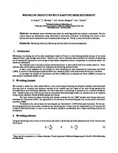
In this study, the Harten wavelet modified by Sj¨ogreen and Yee18 is used where the wavelet and scaling coefficients at the lowest level are given by 1 (uj−1 + uj+1 ) (45) 2 1 D(0) uj = − (uj−1 − 2uj + uj+1 ) (46) 2 The shapes of the wavelet and scaling functions can be computed from the cascade algorithm and are shown in Figure 2. A(0) uj

=

0.7 0.6 0.6 0.4

0.5 0.4

0.2 Φ

Ψ

0.3 0

0.2 −0.2

0.1 0

−0.4

−0.1 −0.6 −2

−1.5

−1

−0.5

0 x

0.5

1

1.5

−0.2 −2

2

−1.5

−1

(a) Wavelet function

−0.5

0 x

0.5

1

1.5

2

(b) Scaling function

Figure 2. Harten wavelet and scaling functions

Wavelet coefficients in two-dimensional space are estimated from the one-dimensional wavelet coefficients in different directions. For example, if the one-dimensional wavelet coefficients in a two-dimensional space are Z ∞ (m) (m) (wx )i,j = u(x, y)ψi (x)dx (47) −∞ Z ∞ (m) (m) (wy )i,j = u(x, y)ψj (y)dy (48) −∞

the two-dimensional wavelet coefficients are estimated from rn o2 n o2 (m) (m) (m) wi,j = (wx )i,j + (wy )i,j

(49)

We define the first version of the wavelet detectors as the wavelet coefficients normalized by the local ”mean” of the scaling coefficients at one lower level (m)

(m) w ˜i,j

w i,j = (m−1) mean ui,j + (i,j)∈S


(50)

The local ”mean” of the scaling coefficients of Harten wavelet is defined as 1 rn o2 n o2 (m) (m) (m) (m) (m) (m) (m) ui+1,j + 2ui,j + ui−1,j + ui,j+1 + 2ui,j + ui,j−1 mean ui,j = 2 (i,j)∈S

(51)

(m)

If w ˜i,j at any level is greater than a user-defined tolerance tollocal , the corresponding cell is tagged for refinement. It should be noted that the local ”mean” is designed in a way that if the detector is only applied to one level of scale, the Harten wavelet detector will reduce to Jameson’s gradient detector because (1) w ˜i,j = w ˜i,j . The wavelet coefficients also have a property that if ψ(x) is compact and if they satisfy max

(m)

j∈S(x0 ,m)

| < u, ψj+k > | ≤ C2mα

(52)

then the solutions at x = x0 satisfy α

|u(x) − u(x0 )| ≤ C |x − x0 |

(53)

where α is the Lipschitz exponent that measures the local regularity or smoothness of the solutions. The higher the value of α, the smoother the solution is locally. The regularity condition is also valid for higher dimensional wavelet coefficients. According to previous literature,19 the local regularity can be estimated from the least square fit of the wavelet coefficients: (m)

log2 rj (m)

where rj

= αj m + c

(54)

is the maximum of the wavelet coefficients over the domain of dependence (m)

rj

=

max

k=−2m p,2m q

(m)

| < u, ψj+k > |

(55)

With the estimated local regularity αj , one can define the second version of wavelet detector by adding one more constraint to the first version that cell is only tagged if αj is also smaller than a tolerance tolα .

V.

Numerical Results and Comparison

Results of four inviscid test problems are presented in this section to examine the performance of the AMR method with the three error detectors: gradient detector, multiresolution detectors with and without constraint on local regularity. The third order total variation diminishing Runge-Kutta scheme20 (RK-TVD) is used for time integration. The implementation of Runge-Kutta scheme in AMR algorithm follows Pantano et al.5 A.

Two-dimensional Kelvin-Helmholtz instability

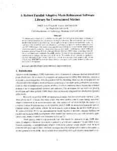
The first test problem is the single-species two-dimensional Kelvin-Helmholtz instability problem which was designed by McNally et al.21 Figure 3 shows the schematic of the initial flow field and the computational domian of the problem. The problem has a periodic domain of size [0, D] × [0, D] which consists of two shear layers at y = 1/4D and y = 3/4D. The initial density and shear velocity in the x direction u are given by   −y/D+3/4 −y/D+3/4   L/D L/D , if 1 > y/D ≥ 3/4 , if 1 > y/D ≥ 3/4 ρ − ρ e   1 m u1 − um e    y/D−3/4 y/D−3/4    ρ + ρ e L/D , L/D u2 + um e if 3/4 > y/D ≥ 1/2 , if 3/4 > y/D ≥ 1/2 2 m u= ρ= −y/D+1/4 −y/D+1/4     u2 + um e L/D , if 1/2 > y/D ≥ 1/4 ρ2 + ρm e L/D , if 1/2 > y/D ≥ 1/4   y/D−1/4 y/D−1/4     ρ1 − ρm e L/D , if 1/4 > y/D ≥ 0 u1 − um e L/D , if 1/4 > y/D ≥ 0 where ρm = (ρ1 + ρ2 )/2 and um = (u1 + u2 )/2. The velocity in the y direction v is perturbed by v φx = λ sin( ) um D 10 of 26 American Institute of Aeronautics and Astronautics

(56)

ρ1 = 1.0, ρ2 = 2.0, u1 = 0.5, u2 = −0.5, L = 0.025, D = 1.0, λ = 0.02 and φ = 4π are chosen in this work. The pressure is initially uniform in space with value 2.5. The ratio of specific heats of the gas is γ = 5/3. All cases in this section are run with CFL = 0.5 and the numerical scheme is set with parameters C = 1.0e8, β TV p = 2, q = 4, αRL = 2.0 and αRL = 50.0. Figure 4 shows the density contours of the reference solution computed on a uniform grid with resolution of 2048 × 2048 at different time. From the sub-figures, it can be seen that the instability grows in linear regime initially from t = 0 to t = 0.75. From t = 0.75 to t = 1.5, the instability emerges into the nonlinear regime and billows of vortices are observed. At t = 1.5, no secondary Kelvin-Helmholtz billows due to numerical oscillations are formed and this observation matches the results of McNally et al.21 D

ρ1 , u 1

λum

v

ρ2 , u 2

D

y ρ1 , u 1

x

Figure 3. Schematic diagram of initial flow field and computational domain of 2D Kelvin-Helmholtz instability problem.

AMR simulations using the three error detectors with different settings are conducted and compared. All AMR simulations have three levels of grids with a root grid resolution of 128×128. A constant 1:2 refinement ratio is used among all grid levels. Three levels of scales are used for the multiresolution detectors. The weighted total numbers of cells and the L2 errors of all cases at t = 1.5 are shown in Tables 1, 2 and 3. The weighted total number of cells is the sum of the cells at different levels weighted by the grid level as at higher levels have smaller time steps and consume more computational power. It is defined as Plgrids max ∆xlmax l=0 ∆xl Nl , where Nl is the number of cells at level l. The weighted total number of cells can be used as the estimation of the computational cost since we notice that in all test problems the cost of convective flux computation, which is dependent on the weighted total number of cells, accounts for the largest portion of total cost while the cost in feature detection is generally less than 1% of total cost. Two different L2 errors are reported in the tables. ”L2 error of root grid” is the L2 error computed from the AMR solutions of the root grid relative to the reference solution projected to the root grid. ”L2 error” is the L2 error computed from the AMR solutions projected to the highest grid level relative to the reference solution projected to the same grid level. Both L2 errors are computed based on the density. From the tables, we observe that as we decrease the value of threshold tollocal in each error detector, both L2 errors decrease. As for the multiresolution detector with constraint on local regularity, we can see in Table 3 that the L2 errors decrease with the increase of tolα as expected since a larger tolα is equivalent to a more strict requirement on the local regularity or smoothness of the solution. In general, the decrease in L2 errors has the trade-off of increment in the number of cells at each refinement level. In order to see the effect of extending the gradient detector to the multiresolution detector, we should compare all detectors with the same value of tollocal . With the same value of tollocal , the L2 errors of multiresolution detector without constraint on local regularity are generally an order of magnitude smaller compared to the gradient sensors. If we only focus on the multiresolution sensor with constant threshold tolα = 1.6, the detector generally produces slightly larger errors than the multiresolution sensor without tolα but with a large amount of savings on the number of refined cells. It should be noted that a simulation with uniform grid spacing as that of the highest level in the AMR simulations has 262144 cells and the L2 error is 3.706E-03. Figures 5, 6 and 7 show the comparison of the refined regions between the three error detectors. Each figure consists of sub-figures of density profiles at t = 1.5 computed from AMR simulations using error detectors with the same value of tollocal , where the multiresolution detector with constraint on local regularity has tolα = 1.6. The boxes in the figures indicate the location of refinement at different grid levels. It can be seen that all sensors can identify the shear layers for refinement. With the same value of tollocal , both 11 of 26 American Institute of Aeronautics and Astronautics

multiresolution detectors identify larger regions to refine compared to the gradeint detector since the two multiresolution detectors are extension of the gradient detector to identify features of more than one scale. The multiresolution detector with the constraint on local regularity refines a smaller domain compared to the one without constraint and this is also reflected in the number of refined cells in the tables.

(a) t = 0.0

(b) t = 0.75

(c) t = 1.5

Figure 4. Density of 2D Kelvin–Helmholtz instability problem computed with uniform grid resolution of 2048 × 2048 at different time. Contours are from 1.0 to 2.0.

tollocal

number of cells on root grid

number of cells on level 1


weighted total number of cells

L2 error of root grid

L2 error

0.01 0.006 0.004

128x128 128x128 128x128

10592 13700 15404

17624 21168 24376

27016 32114 36174

1.480E-02 1.345E-02 1.148E-02

1.563E-02 1.338E-02 1.162E-02

Table 1. Number of cells at different grid levels and L2 errors based on density of different AMR cases using gradient error detector at t = 1.5 of 2D Kelvin-Helmholtz instability problem.

tollocal






L2 error

0.01 0.006 0.004

128x128 128x128 128x128

27984 31100 33296

62120 70288 80936

80208 89934 101680

7.209E-03 5.117E-03 4.879E-03

6.484E-03 4.133E-03 3.588E-03

Table 2. Number of cells at different grid levels and L2 errors based on density of different AMR cases using multiresolution error detector without threshold tolα at t = 1.5 of 2D Kelvin-Helmholtz instability problem. Detector uses 3 levels of scales.

tollocal

tolα






L2 error

0.01 0.01 0.01

0.6 1.0 1.6

128x128 128x128 128x128

16916 17004 19708

25956 32128 39192

38510 44726 53142

1.345E-02 1.114E-02 7.330E-03

1.411E-02 1.120E-02 6.777E-03

0.006 0.006 0.006

0.6 1.0 1.6

128x128 128x128 128x128

15140 17136 20580

26452 32412 40400

38118 45076 54786

1.463E-02 1.244E-02 5.768E-03

1.529E-02 1.272E-02 4.736E-03

0.004 0.004 0.004

0.6 1.0 1.6

128x128 128x128 128x128

16856 18232 20560

26208 32488 40836

38732 45700 55212

1.452E-02 1.076E-02 5.257E-03

1.516E-02 1.092E-02 4.214E-03

Table 3. Number of cells at different grid levels and L2 errors based on density of different AMR cases using multiresolution error detector with threshold tolα at t = 1.5 of 2D Kelvin-Helmholtz instability problem. Detector uses 3 levels of scales.


(a) gradient detector

(b) multiresolution detector without tolα

(c) multiresolution detector with tolα = 1.6

Figure 5. Density of 2D Kelvin–Helmholtz instability problem at t = 1.5 obtained from AMR simulations using different error detectors. Contours are from 1.0 to 2.0. All detectors have thresholds tollocal = 0.01. Refined regions are shown with boxes. Green boxes: first level of refinement; red boxes: second level of refinement.




Figure 6. Density of 2D Kelvin–Helmholtz instability problem at t = 1.5 obtained from AMR simulations using different error detectors. Contours are from 1.0 to 2.0. All detectors have thresholds tollocal = 0.006. Refined regions are shown with boxes. Green boxes: first level of refinement; red boxes: second level of refinement.




Figure 7. Density of 2D Kelvin-Helmholtz instability problem at t = 1.5 obtained from AMR simulations using different error detectors. Contours are from 1.0 to 2.0. All detectors have thresholds tollocal = 0.004. Refined regions are shown with boxes. Green boxes: first level of refinement; red boxes: second level of refinement.


B.

Two-dimensional shock-vortex interaction

This is a single-species two-dimensional shock-vortex interaction problem that was studied in several previous works.22–24 We study the inviscid version of this problem that consists of a Mach 1.2 stationary shock and a strong vortex initially. The initial configuration and computation domain are shown in Figure 8. The domain has size [0, D] × [0, D]. Initially, the stationary shock is at x = 0 and the vortex is located at (0.05D, 0) upstream of the shock. The initial conditions of the vortex are given by ρ p

= =

1− 1 γ

2 1 (γ − 1) Mv2 e1−(r/R) 2

1 γ−1

γ γ−1 1 2 1−(r/R)2 1 − (γ − 1) Mv e 2 2

1

δu = −Mv e 2 (1−(r/R) ) (y − yv )/(0.0125D) δv

1

2

= Mv e 2 (1−(r/R) ) (x − xv )/(0.0125D)

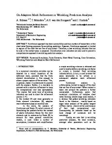
Mv = 1.0, R = 1.0 and D = 80.0 are chosen in this paper. The ratio of specific heats is γ = 1.4. Periodic boundary conditions are applied in the y direction. Dirichlet boundary conditions are used at the right boundary and constant extrapolation is used at the left boundary. All cases in this section are run with TV = 2.0 and CFL = 0.5 and the numerical scheme is set with parameters C = 1.0e8, p = 2, q = 4, αRL β αRL = 50.0. Figure 9 shows the time evolution of the sound pressure dp = (p − p∞ )/p∞ of the reference solution computed with a uniform grid resolution of 4096 × 4096 , where p∞ is the ambient pressure of the post-shock flow. As we can see from the figure, after the vortex interacts with the incident shock, the shock is distorted into an S shape. The primary interaction between the vortex and the incident shock creates reflected shock which has secondary interaction with the deformed vortex and produce more reflected shocks and shocklets. At t = 16.0, we can see the multiple sound waves and reflected shocks that are produced from the multistage interactions. Similar to the two-dimensional Kelvin-Helmholtz instability problem, AMR simulations using the three error detectors with different thresholds are conducted and compared. All of the error detectors are based on pressure and all AMR simulations have three levels of grids with a root grid mesh resolution of 256 × 256. A constant 1:2 refinement ratio is used among all grid levels in all cases. Three levels of scales are used for the multiresolution detectors. Tables 4, 5 and 6 show the number of cells and pressure-based L2 errors of the three error detectors with different settings. From the table, we can notice that all of the L2 errors have same order of magnitude even though different error detectors or thresholds are used. This is due to the fact that the errors around the stationary shock are almost the same in all of the cases and the L2 errors are dominated by the large errors around the stationary shock. However, the slight differences between the L2 errors are sufficient to compare different error detectors. From the tables, we can see that L2 errors decrease with tollocal in all error detectors, similar to the previous test problem. The decrease in L2 is due to more refinement, which is reflected in the increase in the number of cells at different grid levels. As for multiresolution sensor with the constraint on local regularity, the L2 errors decrease with the increase in tolα . It should also be noted that a simulation with uniform grid spacing as that of the highest level in the AMR simulations has 1048576 cells and the L2 error is 1.268E-03. Figures 10, 11 and 12 compare the refined regions between the three error detectors. Each figure consists of sub-figures of sound pressure profiles at t = 16.0 of the three detectors, where the multiresolution detector with the constraint on local regularity has tolα = 1.6. All detectors in the same figure use the same threshold tollocal . On top of the figures are boxes that show the regions of refinement. From the figures, it can be seen that all sensors are able to identify regions around the deformed vortex and stationary shock for refinement. If we decrease tollocal of a particular sensor, more regions around features such as reflected shocks and acoustic waves are refined. It is also clear that using the same value for tollocal , gradient detector generally identifies the smallest regions for refinement and multiresolution detector without constraint on local regularity refines the most. Figure 13(a) shows the global radial profile of the sound pressure from the center of vortex of all error detectors with tollocal = 0.004 at t = 16.0 and θ = −45.0o , compared with the reference solution of Chatterjee et al.,24 which is computed from a ninth order WENO scheme. Figure 13(b) shows the ”zoomed in” region 14 of 26 American Institute of Aeronautics and Astronautics

around a reflected shock at x ≈ 14.0. We can observe that results from both multiresolution detector are very similar near the reflected shock and are more accurate in capturing the sharpness and location of the reflected shock compared with the gradient detector. 0.875D

0.125D

Post-shock

y

Pre-shock

vortex

D

θ r (x , y ) v v = (0.05D, 0)

x

Figure 8. Schematic diagram of initial flow field and computational domain of 2D shock-vortex interaction problem.

(a) t = 4.0

(b) t = 8.0

(c) t = 16.0

Figure 9. Sound pressure of the 2D shock-vortex interaction problem computed with a uniform grid resolution of 4096 × 4096 at different time. Contours are from -0.05 to 0.05.

tollocal






L2 error

0.006 0.004 0.002

256x256 256x256 256x256

5852 7732 12640

11892 12740 20116

31202 32990 42820

2.921E-03 2.890E-03 2.815E-03

1.553E-03 1.491E-03 1.346E-03

Table 4. Number of cells at different grid levels and L2 errors based on pressure of different AMR cases using gradient error detector at t = 16.0 of 2D shock-vortex interaction problem.

tollocal






L2 error

0.006 0.004 0.002

256x256 256x256 256x256

20868 24000 38996

40508 44976 72164

67326 73360 108046

2.877E-03 2.850E-03 2.791E-03

1.448E-03 1.388E-03 1.259E-03

Table 5. Number of cells at different grid levels and L2 errors based on pressure of different AMR cases using multiresolution error detector without threshold tolα at t = 16.0 of 2D shock-vortex interaction problem. Detector uses 3 levels of scales.


tollocal

tolα






L2 error

0.006 0.006 0.006

0.6 1.0 1.6

256x256 256x256 256x256

11568 13996 11684

18072 19488 22864

40240 42870 45090

4.406E-03 3.454E-03 2.908E-03

3.801E-03 2.647E-03 1.530E-03

0.004 0.004 0.004

0.6 1.0 1.6

256x256 256x256 256x256

12512 13112 14668

19636 23580 25880

42276 46520 49598

4.350E-03 3.218E-03 2.860E-03

3.737E-03 2.138E-03 1.438E-03

0.002 0.002 0.002

0.6 1.0 1.6

256x256 256x256 256x256

17304 22676 27284

26244 39676 48268

51280 67398 78294

4.205E-03 3.257E-03 2.805E-03

3.448E-03 2.206E-03 1.296E-03

Table 6. Number of cells at different grid levels and L2 errors based on pressure of different AMR cases using multiresolution error detector with threshold tolα at t = 16.0 of 2D shock-vortex interaction problem. Detector uses 3 levels of scales.




Figure 10. Sound pressure of 2D shock-vortex interaction problem at t = 16.0 obtained from AMR simulations using different error detectors. Contours are from -0.05 to 0.05. All detectors have thresholds tollocal = 0.006. Refined regions are shown with boxes. Green boxes: first level of refinement; red boxes: second level of refinement.




Figure 11. Sound pressure of 2D shock-vortex interaction problem at t = 16.0 obtained from AMR simulations using different error detectors. Contours are from -0.05 to 0.05. All detectors have thresholds tollocal = 0.004. Refined regions are shown with boxes. Green boxes: first level of refinement; red boxes: second level of refinement.





Figure 12. Sound pressure of 2D shock-vortex interaction problem at t = 16.0 obtained from AMR simulations using different error detectors. Contours are from -0.05 to 0.05. All detectors have thresholds tollocal = 0.002. Refined regions are shown with boxes. Green boxes: first level of refinement; red boxes: second level of refinement. 0.05

0.035

0.04

0.03

0.03 0.025 0.02 0.02 ∆p

∆p

0.01 0

0.015

−0.01

0.01

−0.02 0.005 −0.03 0

−0.04 −0.05 0

5

10 r

15

20

−0.005 12

13

14

15

16

17

18

19

r

(a) Global profile

(b) Local profile

Figure 13. Radial variation of sound pressure at θ = −45o computed with AMR simulations using different error detectors. All detectors have thresholds tollocal = 0.004. Red dashed line: gradient detector; green dotted line: multiresolution detector without tolα ; blue dash-dot line: multiresolution detector with tolα = 1.6; black circles: reference solution of Chatterjee et al.24

C.

Two-dimensional shock-bubble interaction

This is a two-species and two-dimensional problem of a shock-bubble interaction by Shankar et al.25 with the domain size of [0, 6.5D] × [−0.89D, 0.89D]. A helium bubble of size D is initially located at [3.5D, 0] in stationary pre-shock air. A Mach 1.22 normal shock that is launched at position x = 4.5D moves to the left to interact with the bubble. After the shock has interacted with the bubble, the interface between the helium and air deforms due to the baroclinic torque. The initial conditions are given by  T  for pre-shock air  (1.0, 0.0, 0.0, 1.0/1.4, 1.4) , T

(ρ, u, v, p, γ) =

T

(1.3764, −0.3336, 0.0, 0.0, 1.5698/1.4, 1.4) , for post-shock air    T (0.1819, 0.0, 0.0, 1.0/1.4, 1.648) , for helium bubble

Slip-wall boundary conditions are applied on the upper and lower boundaries respectively. Both left and right boundary conditions are extrapolated from the interior domain. The initial flow field and computational domain are shown in Figure 14. In order to minimize grid-dependent features, the initial material interface


is smoothed with an artificial diffusion layer between the fluids. The diffusion layer is given by 1 ∆R (1 + erf ( )) 2 i v = vL (1 − fsm ) + vR fsm

fsm =

(57)

where v are any primitive variables (partial density, velocity, pressure and volume fraction) near the initial interface and should not be confused with the symbol of velocity in the y direction. Subscripts L and R denote the left and right interface conditions. erf is the error function. ∆R is the distance from the initial perturbed material interface. i is the characteristic length of the interface thickness that controls the number of grid points across the material interface. Greater value of i implies thicker initial material interface. i = 0.0075 is chosen for all simulation cases in this two-dimensional problem. The domain is set TV with D = 1.0 and the numerical scheme is tuned with parameters C = 1.0e10, p = 2, q = 4, αRL = 2.0 and β αRL = 50.0. All simulations are run with CFL = 0.4. Three AMR simulations are conducted using the three different error detectors. In this problem, error detectors are based on both density and pressure to capture material interfaces and shocks respectively. tollocal of density and pressure are set to 0.05 and 0.01 respectively in all the sensors. The multiresolution detector with constraint on local regularity has tolα = 1.6. All multiresolution detectors are based on three levels of scales. The refinement ratio is set to 1:2 and 5 levels of grids are used with the root grid resolution of 325 × 89. Figure 15 shows the bubble structure of the reference solution computed on a uniform grid with resolution of 2600 × 712 at different time. The upper parts of the sub-figures are contours of the nonlinear function of density gradient magnitude, φ = exp (|∇ρ| / |∇ρ|max ) and the lower parts are the vorticity contours. From Figures 16 and 17, we can compare the solutions from AMR simulations using the three different error detectors at t = 1.0 and t = 6.0. Clearly, all detectors can successfully identify regions near the discontinuities at t = 1.0. The two multiresolution detectors tag more cells around the discontinuities for refinement due to their more global behavior in feature detection. At t = 6.0, the difference between the error detectors is significant as it can be seen that the gradient detector is weaker at identifying regions for refinement in the bubble that contain vortical features and those features are seriously dissipated due to insufficient mesh resolution. Compared to the gradient error detector, both multiresolution detectors can capture almost all of the vortical features compared to the reference solution, which is computed on a grid equivalent to the finest level grid of the AMR simulations when the whole domain is refined to the finest level. In Figure 18, 2 we can see the mean of the enstrophy, Ω = ρ |ω| , where ω is the vorticity, and the weighted total number of cells over time. From the enstrophy plot, it can be seen that the AMR simulations with multiresolution detectors can predict the growth of enstrophy due to baroclinic torque from the interaction between shocks and the material interfaces well until t ≈ 4.5 compared to the reference solution. The gradient detector can only predict the growth of enstrophy well until t ≈ 2.5 before vortices due to secondary instabilities start to grow. However, simulations with the multiresolution detectors consume more computational resources as more cells are refined compared to the gradient detector. Nevertheless, the multiresolution detector with constraint on local regularity can reduce a fraction of cells while the effect of the constraint on the prediction of the time evolution of enstrophy is small. 6.5D y Pre-shock

Air

Helium bubble

x

D

Post-shock 1.78D

0.5D

2D

Figure 14. Schematic diagram of initial flow field and computational domain of 2D shock-bubble interaction problem.


(a) t = 0.5

(b) t = 1.0

(c) t = 1.5

(d) t = 3.0

(e) t = 4.5

(f) t = 6.0

Figure 15. Computed solutions of 2D shock-bubble interaction problem with a uniform grid resolution of 2600×712 at different time. Nonlinear function of normalized density gradient magnitude, φ = exp |∇ρ| / |∇ρ|max for upper half, contours from 1.0 to 1.7. Vorticity for lower half, contours from -20.0 to 20.0.




Figure 16. Solutions of 2D shock-vortex interaction problem at t = 1.0 obtained from AMR simulations using different error detectors. Nonlinear function of normalized density gradient magnitude, φ = exp |∇ρ| / |∇ρ|max for upper half, contours from 1.0 to 1.7. Vorticity for lower half, contours from -20.0 to 20.0. Refined regions are shown with boxes. Green boxes: first level of refinement; blue boxes: second level of refinement; red boxes: third level of refinement.





Figure 17. Solutions of 2D shock-vortex interaction problem at t = 6.0 obtained from AMR simulations using different error detectors. Nonlinear function of normalized density gradient magnitude, φ = exp |∇ρ| / |∇ρ|max for upper half, contours from 1.0 to 1.7. Vorticity for lower half, contours from -20.0 to 20.0. Refined regions are shown with boxes. Green boxes: first level of refinement; blue boxes: second level of refinement; red boxes: third level of refinement.

1.5

1.8

x 10

5


1.6

mean(Ω)

1

0.5

1.4 1.2 1 0.8 0.6 0.4

0 0

1

2

3 t

4

5

6

0.2 0

(a) Enstrophy

1

2

3 t

4

5

6

(b) Weighted total number of cells

Figure 18. Time profile of the mean of enstrophy and the weighted total number of cells of 2D shockbubble interaction computed with AMR simulations using different error detectors. Red dashed line: gradient detector; green dotted line: multiresolution detector without tolα ; blue dash-dot line: multiresolution detector with tolα = 1.6; black solid line: reference solution computed with uniform grid resolution of 2600 × 712.

D.

Three-dimensional shock-bubble interaction

This two-species three-dimensional problem has initial conditions and configuration similar to one of the cases by Niederhaus et al.26 The computation domain has a size of [−4R, 4R] × [0, 12R] × [−4R, 4R], which is shown in Figure 19. Initially a Mach 1.68 normal shock is launched at x = Ls . The shock propagates towards a spherical krypton bubble of radius R located at x = (Ls + Lb ) and interacts with it. R = 2.54 cm, Ls = 2.0 cm and Lb = 5.5 cm are chosen. The initial conditions are:  T 3  for pre-shock air   1.205 kg/m , 0.0, 0.0, 0.0, 1.013e5 Pa, 1.399 , T T 3 (ρ, u, v, w, p, γ) = 2.610 kg/m , 0.0, 310.1 m/s, 0.0, 3.166e5 Pa, 1.399 , for post-shock air   T  3.485 kg/m3 , 0.0, 0.0, 0.0, 1.013e5 Pa, 1.672 , for krypton bubble where u, v, and w are velocity components in the x, y an z directions. Constant extrapolations are applied on all the faces. The initial material interface is smoothed with Eq.57 and i = 595µm. The numerical 20 of 26 American Institute of Aeronautics and Astronautics

β TV scheme is set with parameters C = 1.0e10, p = 2, q = 4, αRL = 2.0 and αRL = 50.0 and CFL is set to 0.4 for all cases in this problem. Three sets of AMR simulations are performed using the three error detectors. Each set has three simulations with root grid resolutions 8 × 16 × 8, 16 × 24 × 16, and 32 × 48 × 32 respectively. All error detectors are based only on density since the initial density ratios across the incident shock wave and material interface are very close. tollocal = 0.04 is set for all error detectors and the multiresolution detector with constraint on local regularity has tolα = 1.6. All AMR simulations have 5 levels of grids and 1:2 refinement ratio. Figure 20 shows the bubble structure of the AMR simulation computed with multiresolution detector without constraint on regularity on a root grid with resolution of 32 × 48 × 32 on the x-y plane at different non-dimensional time τ . τ is defined as τ = tWi /R, where t is the time after the shock starts to interact with the bubble interface and Wi is the incident shock speed. The upper parts of the sub-figures are contours of the nonlinear function of density gradient magnitude, φ = exp (|∇ρ| / |∇ρ|max ) and the lower parts are the contours of z-component of vorticity normalized by its maximum magnitude over the domain. As we can see from the figures, after the passage of the shock, a very significant vortex core is produced and grows with time. An upstream and a downstream jet are also produced due to shock focusing and strong reflections. Figures 25 and 26 show the 3D views of the refined regions and iso-surfaces of mass fractions and vorticity magnitude of the three detectors at τ = 8.0. Figure 21 shows a more detailed comparison of the solutions from different error detectors with root grid resolution of 32 × 48 × 32 at τ = 1.0 and τ = 10.0. From the sub-figures of τ = 1.0 which corresponds to the time when the shock is passing through the bubble, we can see that all error detectors can identify locations of shocks and material interfaces for refinement. At later time τ = 10.0, it is evident that both multiresolution sensors can capture the vortical features better, especially the downstream jet, as we can see that in the case with gradient detector, the downstream jet is heavily dissipated because of insufficient mesh refinement, while the same feature is well preserved in the two cases with multiresolution detectors. However, the two multiresolution detectors are less local in refining regions near discontinuities at earlier time such as τ = 1.0. This behavior is also observed in all other test problems. Figure 22 shows the convergence of the quantity circulation Γ, which is defined as Z ymax Z zmax Z Z 1 ymax 0 (58) + ω (x = 0)dzdy ω (x = 0)dzdy Γx = x x 2 ymin 0 ymin zmin Z ymax Z xmax Z Z 1 ymax 0 Γz = (59) ωz (z = 0)dxdy ωz (z = 0)dxdy + 2 ymin

Γ

=

ymin

xmin

0

1 (Γx + Γz ) 2

(60)

where ωx and ωz are vorticity components in the x and z directions. From the figure, we can see that both multiresolution detectors have good convergence behavior within the time domain shown. The multiresolution detector with the constraint on local regularity has slightly better convergence. However, we cannot observe clear convergence of circulation after τ = 2.5 for the gradient detector. In Figure 23, the results of the three error detectors with root grid resolution of 16 × 24 × 16 are compared. It is obvious that the circulation computed by gradient detector is the worst compared to the reference solution due to its poorer performance in capturing vortical features. Figure 24(a) and 24(b) compare time evolution of the weighted total number of cells of different error detectors with two different mesh resolutions 16 × 24 × 16 and 32 × 48 × 32. Both figures reveal that the multiresolution detector without constraint on local regularity refines the most and the gradient detector has the least amount of refined cells. The multiresolution detector with constraint on local regularity minimizes the number of redundant refined cells while we cannot see any significant difference between the two multiresolution detectors in the prediction of circulation growth.


Post-shock air Ls Lb

8R

Krypton bubble Pre-shock air R

8R

x y z

12R

Figure 19. Schematic diagram of initial flow field and computational domain of 3D shock-bubble interaction problem.

(a) τ = 1.6

(b) τ = 2.6

(c) τ = 5.0

(d) τ = 10.0

Figure 20. Solutions of 3D shock-bubble interaction problem computed with 5-level AMR simulations with multiresolution error detector without tolα with root grid resolution of 32 × 48 × 32 at different time. All levels have 1:2 refinement ratio. Nonlinear function of normalized density gradient magnitude, φ = exp |∇ρ| / |∇ρ|max for upper half, contours from 1.0 to 1.7. Vorticity in the z direction normalized by maximum vorticity for lower half, contours from -3.0 to 3.0.


(a) τ = 1.6, gradient detector

(b) τ = 10.0, gradient detector

(c) τ = 1.6, multiresolution detector without tolα

(d) τ = 10.0, multiresolution detector without tolα

(e) τ = 1.6, multiresolution detector with tolα = 1.6

(f) τ = 10.0, multiresolution detector with tolα = 1.6

Figure 21. Solutions of 3D shock-bubble interaction problem computed with AMR simulations using different error detectors with root grid resolution of 32 × 48 × 32 at different time. Nonlinear function of normalized density gradient magnitude, φ = exp |∇ρ| / |∇ρ|max for upper half, contours from 1.0 to 1.7. Vorticity in the z direction normalized by maximum vorticity for lower half, contours from -3.0 to 3.0. Refined regions are shown with boxes. Yellow boxes: first level of refinement; green boxes: second level of refinement; blue boxes: third level of refinement; red boxes: fourth level of refinement.


8

8

8

6

6

6 Γ

10

Γ

10

Γ

10

4

4

4

2

2

2

0 −1

0 0

1

2

3 τ

4

5

6

7

0

−1


0

1

2

3 τ

4

5

6

7

−1

0

1

2

3 τ

4

5

6

7

(b) multiresolution detector without tolα (c) multiresolution detector with tolα = 1.6

Figure 22. Convergence of time profile of circulation Γ of 3D shock-bubble interaction problem computed with AMR simulations using different error detectors with different root grid resolutions. Red dashed line: 8 × 12 × 8; green dotted line: 16 × 24 × 16; blue dash-dot line: 32 × 48 × 32.

10

8

Γ

6

4

2

0 −1

0

1

2

3 τ

4

5

6

7

Figure 23. Comparison of time profile of circulation o 3D shock-bubble interaction Γ computed with different error detectors on a root grid with resolution 16 × 24 × 16. Red dashed line: gradient detector; green dotted line: multiresolution detector without tolα ; blue dash-dot line: multiresolution detector with tolα = 1.6; black solid line: solution computed from AMR simulation using multiresolution detector with tolα = 1.6 with a root grid resolution of 32 × 48 × 32.

3.5

x 10

6

16



6

14

3

2.5

2

1.5

1

0.5

x 10

12 10 8 6 4

0

2

4

6

8

10

2

0

2

4

τ

6

8

10

τ

(a) Root grid resolution: 16 × 24 × 16

(b) Root grid resolution: 32 × 48 × 32

Figure 24. Time profile of the weighted total number of cells of 3D shock-bubble interaction computed with AMR simulations using different error detectors with two different root grid resolutions of 16 × 24 × 16 and 32 × 48 × 32. Red dashed line: gradient detector; green dotted line: multiresolution detector without tolα ; blue dash-dot line: multiresolution detector with tolα = 1.6.





Figure 25. Refined regions of 3D shock-bubble interaction problem with root grid resolution of 32 × 48 × 32 at τ = 8.0 obtained from AMR simulations. Yellow boxes: first level of refinement; green boxes: second level of refinement; blue boxes: third level of refinement; red boxes: fourth level of refinement.




Figure 26. Iso-volumes and iso-surfaces of 3D shock-bubble interaction problem at τ = 8.0 obtained from AMR simulations with root grid resolution of 32 × 48 × 32. Opaque iso-volumes with a quadrant cut: mass fraction of krypton from 0.2 to 1.0; transparent iso-surfaces: vorticity at value of 8.0e4 s−1 .

VI.

Conclusion

We have discussed the extension of a non-dimensional gradient detector to a multiresolution wavelet detector by sensing gradient of features at multiple scales. The multiresolution detector can be further extended by adding one more constraint on the local regularity estimated from the wavelet coefficients at different scales. We compare the performance of gradient based error detector and two multiresolution detectors for identifying features like shock waves, material interfaces and vortical features in various test problems. The multiresolution detectors outperform the gradient detector in identifying weaker discontinuities and also edges of vortices but with the drawback of refining more cells. The multiresolution detector with the constraint on regularity can be a remedy to reduce the amount of redundant cells due to over-refinement without any appreciable loss in accuracy.

VII.

Acknowledgements

The authors gratefully acknowledge the Institute for Computational and Mathematical Engineering of Stanford University for providing computing time of the high performance MPI clusters. This work also used the Extreme Science and Engineering Discovery Environment (XSEDE),27 which is supported by National


Science Foundation grant number TG-CTS080041N.

References 1 Wong, M. L. and Lele, S. K., “Improved Weighted Compact Nonlinear Scheme for Flows with Shocks and Material Interfaces: Algorithm and Assessment,” AIAA Paper 2016-1807 , 2016. 2 Berger, M. J. and Colella, P., “Local adaptive mesh refinement for shock hydrodynamics,” Journal of computational Physics, Vol. 82, No. 1, 1989, pp. 64–84. 3 Li, S. and Hyman, J., “Adaptive mesh refinement for finite difference WENO schemes,” Los Alamos Report LA-UR-03 , Vol. 89272003, 2003. 4 Baeza, A. and Mulet, P., “Adaptive mesh refinement techniques for high-order shock capturing schemes for multidimensional hydrodynamic simulations,” International Journal for Numerical Methods in Fluids, Vol. 52, No. 4, 2006, pp. 455– 471. 5 Pantano, C., Deiterding, R., Hill, D. J., and Pullin, D. I., “A low numerical dissipation patch-based adaptive mesh refinement method for large-eddy simulation of compressible flows,” Journal of Computational Physics, Vol. 221, No. 1, 2007, pp. 63–87. 6 Wissink, A. M., Hornung, R. D., Kohn, S. R., Smith, S. S., and Elliott, N., “Large scale parallel structured AMR calculations using the SAMRAI framework,” Supercomputing, ACM/IEEE 2001 Conference, IEEE, 2001, pp. 22–22. 7 Hornung, R. D. and Kohn, S. R., “Managing application complexity in the SAMRAI object-oriented framework,” Concurrency and Computation: Practice and Experience, Vol. 14, 2002. 8 Hornung, R. D., Wissink, A. M., and Kohn, S. R., “Managing complex data and geometry in parallel structured AMR applications,” Engineering with Computers, Vol. 22, No. 3-4, 2006, pp. 181–195. 9 Allaire, G., Clerc, S., and Kokh, S., “A five-equation model for the simulation of interfaces between compressible fluids,” Journal of Computational Physics, Vol. 181, No. 2, 2002, pp. 577–616. 10 Johnsen, E. and Colonius, T., “Implementation of WENO schemes in compressible multicomponent flow problems,” Journal of Computational Physics, Vol. 219, No. 2, 2006, pp. 715–732. 11 Coralic, V. and Colonius, T., “Finite-volume WENO scheme for viscous compressible multicomponent flows,” Journal of computational physics, Vol. 274, 2014, pp. 95–121. 12 Nonomura, T. and Fujii, K., “Robust explicit formulation of weighted compact nonlinear scheme,” Computers & Fluids, Vol. 85, 2013, pp. 8–18. 13 Deng, X. and Zhang, H., “Developing high-order weighted compact nonlinear schemes,” Journal of Computational Physics, Vol. 165, No. 1, 2000, pp. 22–44. 14 Taylor, E. M., Wu, M., and Mart´ ın, M. P., “Optimization of nonlinear error for weighted essentially non-oscillatory methods in direct numerical simulations of compressible turbulence,” Journal of Computational Physics, Vol. 223, No. 1, 2007, pp. 384–397. 15 Ren, Y.-X., Zhang, H., et al., “A characteristic-wise hybrid compact-WENO scheme for solving hyperbolic conservation laws,” Journal of Computational Physics, Vol. 192, No. 2, 2003, pp. 365–386. 16 Jameson, A., Schmidt, W., Turkel, E., et al., “Numerical solutions of the Euler equations by finite volume methods using Runge-Kutta time-stepping schemes,” AIAA paper , Vol. 1259, 1981, pp. 1981. 17 Su, X., “Accurate and robust adaptive mesh refinement for aerodynamic simulation with multi-block structured curvilinear mesh,” International Journal for Numerical Methods in Fluids, Vol. 77, No. 12, 2015, pp. 747–766. 18 Sj¨ ogreen, B. and Yee, H., “Multiresolution wavelet based adaptive numerical dissipation control for high order methods,” Journal of Scientific Computing, Vol. 20, No. 2, 2004, pp. 211–255. 19 Mallat, S. and Hwang, W. L., “Singularity detection and processing with wavelets,” Information Theory, IEEE Transactions on, Vol. 38, No. 2, 1992, pp. 617–643. 20 Shu, C.-W. and Osher, S., “Efficient implementation of essentially non-oscillatory shock-capturing schemes, II,” Journal of Computational Physics, Vol. 83, No. 1, 1989, pp. 32–78. 21 McNally, C. P., Lyra, W., and Passy, J.-C., “A well-posed Kelvin-Helmholtz instability test and comparison,” The Astrophysical Journal Supplement Series, Vol. 201, No. 2, 2012, pp. 18. 22 Inoue, O. and Hattori, Y., “Sound generation by shock–vortex interactions,” Journal of Fluid Mechanics, Vol. 380, 1999, pp. 81–116. 23 Zhang, S., Zhang, Y.-T., and Shu, C.-W., “Multistage interaction of a shock wave and a strong vortex,” Physics of Fluids (1994-present), Vol. 17, No. 11, 2005, pp. 116101. 24 Chatterjee, A. and Vijayaraj, S., “Multiple sound generation in interaction of shock wave with strong vortex,” AIAA journal, Vol. 46, No. 10, 2008, pp. 2558–2567. 25 Shankar, S. K., Kawai, S., and Lele, S. K., “Numerical simulation of multicomponent shock accelerated flows and mixing using localized artificial diffusivity method,” AIAA Paper 2010-352 , 2010. 26 Niederhaus, J. H., Greenough, J., Oakley, J., Ranjan, D., Anderson, M., and Bonazza, R., “A computational parameter study for the three-dimensional shock–bubble interaction,” Journal of Fluid Mechanics, Vol. 594, 2008, pp. 85–124. 27 Towns, J., Cockerill, T., Dahan, M., Foster, I., Gaither, K., Grimshaw, A., Hazlewood, V., Lathrop, S., Lifka, D., Peterson, G. D., et al., “XSEDE: accelerating scientific discovery,” Computing in Science & Engineering, Vol. 16, No. 5, 2014, pp. 62–74.


Multiresolution Feature Detection in Adaptive Mesh Refinement with

Multiresolution Feature Detection in Adaptive Mesh Refinement with

Suggest Documents

Feature-Driven Adaptive Mesh Refinement in the

Adaptive Multiresolution Mesh Refinement for the Solution of Evolution

A Hierarchical Multiresolution Adaptive Mesh Refinement for ... - DCSL

adaptive mesh refinement in electromagnetic

Feature-Driven Adaptive Mesh Refinement in the Helios Code

WRINKLING PREDICTION WITH ADAPTIVE MESH REFINEMENT 1

GALAXY MERGERS WITH ADAPTIVE MESH REFINEMENT: STAR ...

Radiation hydrodynamics with Adaptive Mesh Refinement and

Adaptive Mesh Refinement with an automatic hybrid

Adaptive Mesh Refinement applications with CanoP ...

Robust Parallel Adaptive Mesh Refinement

FEATURE-PRESERVING ADAPTIVE MESH

adaptive mesh refinement - Semantic Scholar

COSMOLOGICAL SHOCKS IN ADAPTIVE MESH REFINEMENT

On Adaptive Mesh Refinement in Wrinkling

Optimal imaging with adaptive mesh refinement in electrical ...

Block-Structured Adaptive Mesh Refinement Algorithms and ...

THE GENDARME ALGORITHM FOR ADAPTIVE MESH REFINEMENT

Adaptive Mesh Refinement for Finite Difference

Tutorials on Adapative multiresolution for mesh refinement applied to

AN ADAPTIVE MESH REFINEMENT ALGORITHM FOR ... - CiteSeerX

Parallelization of Structured, Hierarchical Adaptive Mesh Refinement ...

Adaptive Mesh Refinement and Relativistic MHD

Block-structured Adaptive Mesh Refinement - ePrints Soton