IEEE TRANSACTIONS ON SYSTEMS, MAN, AND CYBERNETICS—PART B: CYBERNETICS, VOL. 34, NO. 1, FEBRUARY 2004
499
Adaptive Neural Control of Nonlinear Time-Delay Systems With Unknown Virtual Control Coefficients Shuzhi Sam Ge, Senior Member, IEEE, Fan Hong, Student Member, IEEE, and Tong Heng Lee, Member, IEEE
Abstract—In this paper, adaptive neural control is presented for a class of strict-feedback nonlinear systems with unknown time delays. The proposed design method does not require a priori knowledge of the signs of the unknown virtual control coefficients. The unknown time delays are compensated for using appropriate Lyapunov–Krasovskii functionals in the design. It is proved that the proposed backstepping design method is able to guarantee semiglobal uniformly ultimately boundedness of all the signals in the closed-loop. In addition, the output of the system is proven to converge to a small neighborhood of the origin. Simulation results are provided to show the effectiveness of the proposed approach. Index Terms—Adaptive control, neural networks, nonlinear time-delay systems.
I. INTRODUCTION
R
ECENT years have witnessed great progress in adaptive control of nonlinear systems due to great demands from industrial applications. In order to obtain global stability, some restrictions have to be made to nonlinearities such as matching conditions, extended matching conditions, or growth conditions [1]. To overcome these restrictions, a recursive design procedure called adaptive backstepping design was developed in [2]. Robust adaptive backstepping control has been studied for certain class of nonlinear systems [3]–[5] (to name just a few). While the earlier works such as [3], [4], [6] assumed the virtual control coefficients to be 1, adaptive control has been extended to parametric strict-feedback systems with unknown constant virtual control coefficients but with known signs (either positive or negative) [7] based on the cancellation backstepping design as stated in [8] by seeking for a cancellation of the couin the next step of Lyapunov depling terms related to sign. With the aid of neural network parametrization, adaptive control schemes have been further extended to certain classes of strict-feedback forms in which virtual control coefficients are unknown functions of states with known signs [9], [10]. , the unknown virtual control For system causes great design difficulty in adaptive confunction trol. Based on feedback linearization, certainty equivalent conis usually taken, where and trol are estimates of and , and measures have to be . To avoid taken to avoid controller singularity when this problem, integral Lyapunov functions have been developed
Manuscript received January 29, 2003; revised May 13, 2003. This paper was recommended by Associate Editor H.-X. Li. The authors are with Department of Electrical and Computer Engineering, National University of Singapore (e-mail:
[email protected]). Digital Object Identifier 10.1109/TSMCB.2003.817055
in [9], and semi-globally stable adaptive controllers are developed, which do not require the estimate of the unknown function . Although the system’s virtual control coefficients are assumed to be unknown nonlinear functions of states, their signs are assumed to be known as strictly either positive or negative. Under this assumption, stable neural network controllers have been constructed in [10] by augmenting a robustifying portion, and in [11], [12] by estimating the derivation of the control Lyapunov function. When there is no a priori knowledge about the signs of virtual control coefficients, adaptive control of such systems becomes much more difficult. The first solution was given in [13] for a class of first-order linear systems, where the Nussbaum-type gain was originally proposed. When the high-frequency control gains and their signs are unknown, gains of Nussbaum type [13] have been effectively used in controller design in solving the difficulty of unknown control directions [14], [15] in which the arguments of the constructed Nussbaum functions are required to be monotone increasing. This method was then generalized to higher-order linear systems in [16]. For nonlinear systems, some results have also been reported in the literature. Without the requirement for monotone increasing arguments for the Nussbaum functions, the same technique has been extended to higher order systems for constant virtual control coefficients [17], [18] using decoupled backstepping formally stated in [8] without seeking for the cancellation of the coupling terms rebut to decouple and using Young’s inlated to next. Under the equality and seek for the boundedness of assumption that the virtual control coefficients are time-varying, with unknown signs and bounded in finite intervals, it has also been used to construct robust adaptive control for a class of nonlinear systems with bounded disturbances by introducing exponentially decaying terms to handle the bounded disturbances [19]. The behavior of this class of control laws can be interpreted as the controller tries to sweep all possible control gains and stops when a stabilising gain is found. Another challenging problem in control of nonlinear systems lies in robust control of nonlinear systems with time delays [20], [21]. The existence of time delays may degrade the control performance and make the stabilization problem become more difficult. By using appropriate Lyapunov-Krasovskii functionals [22], uncertainties from unknown time delays can be compensated for. A stabilizing controller design based on the above-mentioned functional was proposed in [23] for a class of nonlinear time-delay systems with a so-called “triangular structure”. However, the uncertainties from unknown parameters or unknown nonlinear functions were not discussed. In [24], we studied a class of nonlinear time-delay systems, in
1083-4419/04$20.00 © 2004 IEEE
500
IEEE TRANSACTIONS ON SYSTEMS, MAN, AND CYBERNETICS—PART B: CYBERNETICS, VOL. 34, NO. 1, FEBRUARY 2004
which the virtual control coefficients are unknown constants with known sign and the system uncertainties are linearly parametrized with unknown constant parameters and known nonlinear functions. Practical stability was introduced to solve the or in singularity problem due to the appearance of the controller and the tracking error can be made to confine in a compact domain of attraction. When the virtual control coefficients are unknown nonlinear functions of states, the problem becomes even more complicated. Although the system’s virtual control coefficients are assumed to be unknown nonlinear functions of states, their signs are assumed to be known as strictly either positive or negative. Under the same assumption, stable neural network controllers have also been constructed in [25] by compensating for the unknown time-delay terms completely are available for feedunder the assumption that signals back and more strict assumption on the time delay terms. Motivated by previous works on both unknown time-delay systems and unknown virtual control coefficient systems, two adaptive neural controllers without the requirements for are presented for a class of strict-feedback nonlinear systems with unknown time delays, and unknown nonlinear functions with unknown signs. For clarity, the first controller is developed based on distinct definitions of two separate compact sets and where “ ” denotes the complement operation. However, the controller has a “technical problem”—the intermediate controls are not differentiable at isolated points . To solve this problem, one practical way is to simply set the differentiation at these points to be any finite value, say 0, and then every signal in the closed-loop system can be shown to be bounded. By modifying the first controller such that the intermediate controls are differentiable, we have the second controller for the class of systems in the paper—which is mathematically rigorous. To the best of our knowledge, there is little work dealing with such a kind of systems in the literature at present stage, except for some preliminary results presented in [25], [26]. The main contributions of the paper lie in: i) the use of integral Lyapunov function in avoiding the controller singularity problem commonly encountered in adaptive feedback linearization control; ii) the combination of Lyapunov-Krasovskii functional and the Young’s inequality in eliminating the unknown time delay in the upper bounding function of the Lyapunov functional derivative, which makes neural network parametrization with known inputs possible; iii) the use of the Nussbaum-type functions in solving the problem of the completely unknown control direction iv) the novel introduction of smooth functions in making the intermediate control laws continuous and differentiable to certain desired order in solving the differentiability problems at some isolated points incurred in the first practical control. The rest of the paper is organized as follows. The problem formulation and preliminaries are given in Section II. An adaptive neural controller design for first-order systems is presented in Section III. The scheme is extended to th-order systems in Section IV. A simulation example is given in Section V, and followed by Section VI which concludes the work.
II. PROBLEM FORMULATION AND PRELIMINARIES Consider a class of single-input-single-output (SISO) nonlinear time-delay systems
(1) where
, , , are the state variables, system input and output reand , are unknown smooth functions, spectively, . The and are unknown time delays of the states, control objective is to design an adaptive controller for system (1) such that the output follows a desired reference signal , while all signals in the closed-loop system are bounded. , Define the desired trajectory , which is a vector of up to its th time derivative . and their signs are unAssumption 1: Functions known, and there exist constants and known smooth such that , functions . take value in Assumption 2: Known smooth functions the unknown closed intervals . , Assumption 3: The desired trajectory vectors are continuous and available, and with known compact sets. Remark 1: Assumption 1 implies that smooth functions are strictly either positive or negative, which is reasonbeing away from zero is the controllable able because condition of system (1), which is made in most control schemes [7], [27]. For a given practical system, the upper bounds of are not difficult to determine by choosing large , the enough. It should be emphasized that the low bounds and are lower and upper bounds of the closed intervals only required for analytical purposes, their true values are not necessarily known. Accordingly, we define positive-definite functions , . From Assumption 1, we know are bounded by known functions as that . Assumption 4: The unknown smooth functions satisfy the inequality where are known positive smooth functions. This assumption is much more relaxed than as has been made in [25]. Assumption 5: The unknown time delays are bounded by a , . known constant, i.e., Remark 2: There are many physical processes which are governed by nonlinear differential equations of the form (1). Examples are recycled reactors, recycled storage tanks and cold rolling mills [21]. In general, most of the recycling processes inherit delays in their state equations.
GE et al.: ADAPTIVE NEURAL CONTROL OF NONLINEAR TIME-DELAY SYSTEMS
A. Nussbaum Type Gain : is a function of NussAny continuous function baum type if it has the following properties:
501
, is th differentiable, i.e., bounded by 1. F2). Even function
and
(6)
(2) is continuous, and monotonic, i.e., for any . positive constant,
, where is a
(3) C. Linearly Parametrized Neural Networks For example, the continuous functions , , and suffice [28]. For clarity, the even Nussbaum is used throughout this function, paper. and be smooth functions deLemma 1: [17] Let with , , and be fined on an even smooth Nussbaum-type function. If the following inequality holds:
where is a nonzero constant and represents some suitable constant, then , and must be . bounded on and be smooth functions defined on Lemma 2: Let with , , and be an even smooth Nussbaum-type function. The following inequality holds:
A function approximator shall be used to approximate the unknown nonlinear functions. There are two basic types of artificial neural networks 1) linearly parametrized neural networks (LPNNs); 2) multilayer neural networks (MNNs). In control engineering, the radial basis function (RBF) neural network (NN) as a kind of LPNNs is usually used as a tool for modeling nonlinear functions because of its nice approximation properties. The RBF NN can be considered as a two-layer network in which the hidden layer performs a fixed nonlinear transformation with no adjustable parameters, i.e., the input space is mapped into a new space. The output layer then combines the outputs in the latter space linearly. Therefore, it belongs to a class of linearly parameterized networks. In this paper, the following RBF NN [29] is used to approximate the continuous function (7) where the input vector
(4) , is a time-varying parameter where constant which takes values in the unknown closed intervals with , and represents some suitable constant, then , and must be bounded on . Proof: See Appendix I. B. Useful Continuous Functions For the construction of differentiable control laws, two continuous functions are introduced as follows. : defined by F1). Even function (5) shown at the bottom of the page, where , and
, weight vector , the NN node number ; and , with being chosen as the commonly used Gaussian functions, , where i.e., is the center of the receptive field and is the width of the Gaussian function. Universal approximation results in [30], [31] indicate that, if is chosen sufficiently large, can approximate any continuous function, , to any desired accuracy over a compact set to , arbitrary any accuracy in the form of where is the ideal constant weight vector, and is the approximation error which is bounded over the , where is an compact set, i.e., is an “artificial” unknown constant. The ideal weight vector is defined as quantity required for analytical purposes. the value of that minimizes for all , i.e., . The stability results obtained in NN control literature are semi-global in the sense that, as long as the input variables of
(5)
502
IEEE TRANSACTIONS ON SYSTEMS, MAN, AND CYBERNETICS—PART B: CYBERNETICS, VOL. 34, NO. 1, FEBRUARY 2004
the NNs remain within some pre-fixed compact set, , can be made as large as desired, there where the compact set exists controller(s) with sufficiently large number of NN nodes such that all the signals in the closed-loop remain bounded. It should be noted that RBF neural networks can be replaced by any linearly parameterized networks without any technical difficulty such as fuzzy systems, polynomial, splines and wavelet networks.
Applying Assumption 4, we have
(11) III. ADAPTIVE CONTROL FOR FIRST-ORDER SYSTEM To illustrate the design methodology clearly, we first consider the tracking problem of a first-order system (8) where
is the control input. Define the tracking error , we have
(9) , and a smooth scalar function
Define
By changing the variable
, we may rewrite . Noting that
Remark 3: It can be seen from (11) that the design difficulties are mainly from two uncertainties: unknown functions , (due to unknown function ) and unknown time is known, state should not delay . Although appear in the designed controller as it is undetermined due to unknown . In addition, the unknown time delay and the unare entangled together in a nonlinear known function fashion, which makes the problem even more complex to solve. Therefore, we have to convert these related terms into such a can be dealt form that the uncertainties from and with separately. By using Young’s Inequality, (11) becomes
as (12)
, we have
(10)
where and are separated and can be dealt with one by one as detailed later. To overcome the design difficulties from the unknown time delay , the following Lyapunov-Krasovskii functional can be considered
Its time derivative is (13) The time derivative of
is
Noting (9) and doing the integration by parts, we have which can be used to cancel the time-delay term on the right hand side of (12) and thus eliminate the design difficulty from the unknown time delay without introducing any uncertainties to the system. For notation conciseness, we will omit the after time-delay terms have been time variables and eliminated. Accordingly, we obtain (14) where
(15)
GE et al.: ADAPTIVE NEURAL CONTROL OF NONLINEAR TIME-DELAY SYSTEMS
with , where is a compact set. At present stage, suppose that the Lyapunov function candi. From (14), we know date is chosen as which is free from unknown that we can design a stabilizing time delay under the assumption of known system functions. is utilized to construct the controller, conNote that if troller singularity may occur since is not well. Therefore, care must be taken to guarantee defined at the boundedness of the control. It is noted that the controller sin, where the control objecgularity takes place at the point tive is supposed to be achieved. From a practical point of view, once the system reaches its origin, no control action should be is hard to detect taken for less power consumption. As owing to the existence of measurement noise, it is more practical to relax our control objective of convergence to a “ball” rather than the origin [24]. and For ease of discussion, let us define sets as (16) (17) where is a constant that can be chosen arbitrarily small and “ ” in (17) is used to denote the complement of set in set as
Lemma 3: Set is a compact set. Proof: See Appendix II. Under the assumption of known system functions, we have the practical robust control law to guarantee the closed-loop stability as detailed in Lemma 4. Lemma 4: For the first-order system (8), if the practical robust control law is chosen as (18)
503
and can be approximated by neural networks compact set to arbitrary any accuracy as (20) where is the approximation error, are unknown ideal constant weights, and are the instead to form the basis functions. Let us use its estimate adaptive control (21) (22) (23) where matrix , and small constant is to introduce the -modification for the closed-loop system. Theorem 1 summarizes the stability result for the proposed adaptive scheme, and shows that certain compact set is a domain of attraction. Theorem 1: Consider the closed-loop systems consisting of the first-order plant (8) and controller (21), (22), if gain with being a design constant, and is chosen as
(24) with constant , and the NN weights are updated by (23), then for bounded initial conditions and , all signals in the closed-loop system are semi-globally uniformly ulremains in a compact set timately bounded, and the vector defined by
(19) where with being any positive constant, then for bounded initial conditions, all the signals in the closed-loop system are globally uniformly ultimately bounded. Proof: See Appendix III. It is shown that the compact set is actually a domain of attraction. Remark 4: For the first-order system, the definition of the in (17) and the corresponding practical control compact set in (18) can guarantee the stability of the closed-loop law system. To extend the above design methodology to higheris not order systems, modification has to be made since . We will discuss this issue at a later differentiable at stage when the problem is clearly shown. and are completely unknown, the In the case that proposed controller (18) in Lemma 4 is not feasible due to the . On the other hand, by employing the unknown function robust control in (18), control action is only activated when . Apparently, is continuous and well-defined over
whose size, , can be adjusted by appropriately choosing the design parameters. Proof: Let us consider the following Lyapunov function candidate (25) where is
. The time derivative of
along (14)
(26) For
, substituting (21) and (23) into (26), we have
(27)
504
IEEE TRANSACTIONS ON SYSTEMS, MAN, AND CYBERNETICS—PART B: CYBERNETICS, VOL. 34, NO. 1, FEBRUARY 2004
Adding and subtracting hand side of (27) and noting (20), we have
on the right
, we can conclude that , and , hence , are . According to Proposition 2 in [15], if the soSGUUB on . Let lution of the closed-loop system is bounded, then be the upper bound of , then we have the following inequalities:
Applying
Lemma
2,
(28) , (28) becomes
Noting
(29) Using the inequalities
Thus, (34) becomes
and substituting (24) into (29), we have
(35) where constant
It follows from (10), (25) and (35) that where (30) Since
according to Assumption 5, inequality holds. From (10)
and (13), we have
(31) where positive constant
is defined by (32)
By letting , we know that . We can readily conclude that there do exist a compact set such that , . Remark 5: If system uncertainties are in the linear-in-the-parameter form as in [17], adaptive control can be used to solve the problem elegantly and the asymptotic stability can be guaranteed by applying Lemma 1. In this paper, the unknown functions are approximated by RBF NN, which has an intrinsic approximation error, therefore Lemma 1 is no longer applicable. To is re-written show the point clearly, the time derivative of as (36)
Letting
and multiplying (31) by
, it becomes
Integrating (36) over
, we have
(33) Integrating (33) over
, we have
(34)
(37) From (37), we cannot draw any conclusion for the boundedness or by applying Lemma 1 in [17] due to the extra of . From the definition of in (30), we know that is term and . a function of NN approximation error Even though we can remove the latter by setting as zero, cannot be the former effect from NN approximation error eliminated. The problem is successfully solved by multiplying to both sides of (36) as did in the proof the exponential term
GE et al.: ADAPTIVE NEURAL CONTROL OF NONLINEAR TIME-DELAY SYSTEMS
of Theorem 1. Consequently, the stability results can be drawn by invoking Lemma 2. Remark 6: Although the system has been proven to converge into a compact set which is actually unknown due to unknown , , , , and , it is possible to adjust the size by and . appropriately choosing design parameters Remark 7: The computation of the second integral of in (24) should be conducted in the time interval . If , the stability the integration is conducted alternatively in result may seem to hold. However, the integral result will progressively tend to a large value as the time increases, which may saturate the actuator and destroy the closed-loop stability. To should avoid this, a rather conservative time interval be chosen for conducting the integration. The same conservative measure will be taken in the later recursive backstepping design. Remark 8: Though it is known that the stability of time-delay systems depends on the size of the time delay, it is not necessarily true for general nonlinear systems as is illustrated by the following example. Consider the linear time-delay system
with , . It has been proven that the linear time delay system is stable if , and the system is unstable if is too large. However, for the forced linear time delay system given by
with
,
, subject to the sliding mode control
505
used to handle the unknown time delays terms as in Section III, different from the classical cases, the Lyapunov function is much more involved, in which the following candidate , and terms appeared times, twice and once respectively rather than a simple summation of the previous ones. The derivations are very troublesome in order to see the choices of the above functionals clearly, and cannot be further simplified because of the nature of the problem. A. Practical Controller Design The backstepping design procedure contains steps. At each shall be developed step, an intermediate control function using an appropriate Lyapunov function . The design of both the control laws and the adaptive laws are based on the fol, , lowing change of coordinates: . Note that the controller design based on such will render not differentiable at points compact sets . This appears to be a “technical problem” as the differentiation of is not defined at these isolated points. To solve this problem, one practical way is to simply set the differentiation at these points to be any finite value, say 0, and then every signal in the closed-loop system can be shown to be bounded. Theoretically speaking, by doing so, there is no much loss either as these points are isolated and can be ignored. For ease and clarity of presentation, we assume that all the control functions are differentiable throughout this subsection. For uniformity of notation, throughout this section, define es, compact sets and as timation errors
we have the resulting nonlinear time delay closed-loop system (38) For the nonlinear time delay system (38), consider the Lyapunov , we have function candidate
Apparently, the nonlinear time delay system (38) is stable for arbitrary . This also verifies the rich dynamic behaviors of nonlinear systems. We have developed a practical adaptive neural control for first-order system (8). Now we are ready to extend the above design methodology to higher-order systems. IV. ADAPTIVE BACKSTEPPING CONTROLLER DESIGN In this section, the adaptive design will be extended to th-order systems (1) and the stability results of the closed-loop system are presented. Note that the extension is not straightforward as in the classical cases of backstepping design for nonlinear systems in strict feedback form without time delays. In the proposed recursive backstepping design, the computation of requires the computation of . As a result, the unknown time-delay terms of all the previous subsystems will appear in Step , which have to be compensated for one by one. Though shall be the idea of Lyapunov-Krasovskii functional
with constants
, and positive constants
,
,
as
where are the estimates of ideal NN weights , are the lower bounds of , constants , , matrices , constants small constants , are the upper bounds of the NN approximation erwith being the corresponding inputs rors, i.e., to be defined later, and the following integral Lyapunov func, the Lyapunov-Krasovskii functionals with tions , and the Lyapunov function the positive scalar functions as candidates (39)
(40)
506
IEEE TRANSACTIONS ON SYSTEMS, MAN, AND CYBERNETICS—PART B: CYBERNETICS, VOL. 34, NO. 1, FEBRUARY 2004
(41)
As stated in Section III, the control objective now is to show that converges to certain domain of attraction rather than the origin. To this end, let us show the derivative of Lyapunov func. Consider the Lyation candidate is nonpositive when given in (42). Its time derivative punov function candidate along (50) is
(42) where positive functions . The adaptive neural control laws are as follows, for
(43)
Choose the practical adaptive neural intermediate control law and NN weights updating law as given in (43)–(45) with given in (46). Now, using the same procedure as in Section III, it can be shown that
(44) (45) where
,
is chosen as
(51) (46) Noting that
, (51) becomes
and are the basis functions with being the input vectors defined in (61) and (68) later. , is actually the control input . Note that when , Step 1: Let us firstly consider the equation in (1) when i.e., (47) From the definition for new states and , we have
and
, i.e., (52) (48)
Consider
in (39). Its time derivative along (48) is
(49)
Remark 9: In the cancellation based backstepping design, the coupling term is left as it is and it will be cancelled in the next step by augmenting the Lyapunv candidate. In decoupled backstepping design, we will not seeking the cancellation , but seeking the boundedness of of the coupling term in the next step. According to Lemma 2, if we could prove that is bounded, then the stability of is apparent and easy. This fundamental change makes control system design for this problem solvable [8]. , we have Since
Following the same procedure as in Section III by choosing in (41) and applying Assumption 4 and Young’s inequality, we obtain (50) where
is defined in (15).
(53)
GE et al.: ADAPTIVE NEURAL CONTROL OF NONLINEAR TIME-DELAY SYSTEMS
Multiplying (53) by
, it becomes
507
Consider
given in (40). Its time derivative is
(54) Integrating (54) over
, we have (58) Noting (57) and
(55) Remark
10: In
(55), if there is no extra term within the inequality, we can conclude , , , are all bounded on according to that and Lemma 2. According to Proposition 2 in [15], we can claim that , are SGUUB. Remark 2.3 in [18] also explains the problem. Due to the presence of extra term in (55), Lemma 2 cannot be applied directly. It was supposed in [17] that if can be regulated such that it is square integrable, the regulation of can be achieved. However, the situation is different in this paper. Owing to the introduction of exponential term in Lemma 2, the requirement for square integrability can be further relaxed to boundedness. Noting Assumption 2, we have the following inequality [18]:
(58) becomes
where
Since is a function of can be expressed as
,
,
,
,
(56) can be regulated as bounded, then from (56) Thus if we can readily conclude the boundedness of the extra term . The effect of will be dealt with in the following steps. : Similar procedures are taken recurStep i . sively for each step of is given by The time derivative of (57)
where
Note that the computation of , which is required by the recursive backstepping design, and the appearance of make
508
IEEE TRANSACTIONS ON SYSTEMS, MAN, AND CYBERNETICS—PART B: CYBERNETICS, VOL. 34, NO. 1, FEBRUARY 2004
the unknown time delays of all the previous subsystems appear, which should all be compensated for in this step. In other words, Lyapunov–Krasovskii functionals (41) shall be utilized to compensate for not only the unknown time delay , but also . This difficulty or complexity was avoided by asis available for feedback control in [25]. suming that Applying Assumption 4 and using Young’s Inequality, we have
(61) For the adaptive neural intermediate control law given in being given in (46), consider Lyapunov (43)–(45) with given in (42). Its time derivative along function candidate (43)–(45) and (60) is (62) Multiplying (62) by
, it becomes
(63) (59)
Integrating (63) over
, we have
where . Considering the Lyapunov-Krasovskii functional given in (41), we have
as
(60) where
(64) Remark 11: Similarly as discussed in Remark 10, if can be regulated as bounded, we can readily guarantee the boundedness of the extra term in (64). Then , , and applying Lemma 2, the boundedness of can be readily obtained. The effect of will be dealt with in the next step.
GE et al.: ADAPTIVE NEURAL CONTROL OF NONLINEAR TIME-DELAY SYSTEMS
Step n. This is the final step, since the actual control appears in the derivative of as given in
Since
is a function of can be expressed as
where
(65) given in (40). Its time
Consider the scalar function derivative is
509
. Considering the Lyapunov-Krasovskii functional given in (41), we have (67) where
,
,
,
,
where
Applying Assumption 4 and using Young’s Inequality, we have
(68) For the adaptive neural control law given in (43)–(45) with being given in (46), consider the Lyapunov function can. Its time derivative along (43)–(45) and (67) is didate (69) Multiplying (69) by
, it becomes
Integrating (70) over
, we have
(70)
(66)
(71)
510
IEEE TRANSACTIONS ON SYSTEMS, MAN, AND CYBERNETICS—PART B: CYBERNETICS, VOL. 34, NO. 1, FEBRUARY 2004
Using Lemma 2, we can conclude that and , hence , are SGUUB on . From the , the boundedness of the extra term boundedness of at Step is readily times backward, it can obtained. Applying Lemma 2 for be seen from the above iterative design procedures that , , and hence are SGUUB, . The following theorem shows the stability and control performance of the closed-loop adaptive system. Theorem 2: Consider the closed-loop system consisting of the plant (1) under Assumptions 1–4, the adaptive neural control laws (43)–(46). We can guarantee the following properties under bounded initial conditions i) all signals in the closed-loop system remain semi-globally uniformly ultimately bounded; remain in the compact set , ii) the vectors ; specified as
whose sizes, , can be adjusted by appropriately choosing the design parameters. Proof: Consider the Lyapunov function candidate given in (42) with , being defined in (40) and (41). From the previous derivation, we have
From the above iterative design procedures from Step 1 to Step , we can conclude , , , , , and are SGUUB. hence Letting be the upper bound of and noting the definition of , we have
In the rest of the steps from
where constant
with for . , we know that By letting . We can conclude that there do exist compact sets such , . that Remark 12: For the choice of in (46), it is found that if is chosen to be very small, will take a very large value, which may saturate the control actuator. To solve this problem, such that it prowe would like to find an alternative for vides smooth control input, and at the same time guarantees the stability result. One such choice is
Following the same derivation procedure and using the property in (6), we can readily obtain (62) with being of function modified/changed to
Although the bounded region may be enlarged by introducing , there are still design flexibility from , the function and , which can help reduce the bounded region. Note that are such modifications together with the choice of function also not unique and worth further investigation. are not unique Remark 13: Note that the choices of [9]. As an alternative, we can choose . In , i.e., are this case, the upper bound function of not necessarily known. The smooth integral scalar function becomes
to 1, we obtain By Mean Value Theorem,
Letting
be the upper bound of and noting the definition of
can be rewritten as
From Assumption 1, , we know that is a positive definite function and . For conciseness of presentation, we give the control and adaptive laws directly without proof, as well as the stability results. Theorem 3: For system (1), we choose the adaptive neural with constant control laws (43)–(45), where and is chosen as , we have
(72)
GE et al.: ADAPTIVE NEURAL CONTROL OF NONLINEAR TIME-DELAY SYSTEMS
511
with , . Then, under the bounded initial conditions, all signals in the closed-loop system remain bounded and the tracking error converges to a small neighborhood around zero by appropriately choosing design parameters. in Remark 12, we can Similar as the modification made to modify (72) to
(73)
for a relatively gentle control gain. B. Differentiable Controller Design Though the nondifferentiability of the intermediate controls can be solved in a very practical way as discussed in the previous subsection. In fact, this problem can also be solved theoretically by modifying the control laws such that they are differentiable to certain desired order as will be discussed below. It should be pointed out that the solution is not unique. For clarity, only one such a solution is presented. requires that of It can be seen that the computation of . This is also the case for the computation of , , and respecand , which requires to compute tively. Therefore, we know that the computation of shall include that of , and . This rule applies to the rest of the steps till the last step . We can conclude that need to be at least th differentiable. By using the propin (5), the inerty of (n-i)th order differentiable function termediate control, in (43) can be easily modified to satisfy th order differentiability as the required
(74) where is defined in (5). It can be easily verified by actual differentiation. The above modification not only guarantees the differentiability of the intermediate controls, but also preserves the closed-loop stability of the practical control design by noticing . In fact, the stability analysis remains that . the same as before for V. SIMULATION
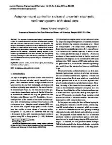
Fig. 1.
Output y (t)(“—”) and reference y (“- -”).
Fig. 2.
Trajectory of state x (t).
Choose the initial condition , the , and the desired reference signal time delay . For the design of neural adaptive controller, let , . For simplicity, simulation is carried out based on Theorem 3 for the case . The intermediate control and control are given by (74) and (43) respectively with being chosen in (73) as
To illustrate the proposed adaptive neural control algorithms, we consider the following second-order time-delay system
otherwise
where
, ,
and and
, , , . Apparently, by choosing , Assumption 4 satisfies.
where the Nussbaum functions,
,
, 2 are ,
512
IEEE TRANSACTIONS ON SYSTEMS, MAN, AND CYBERNETICS—PART B: CYBERNETICS, VOL. 34, NO. 1, FEBRUARY 2004
contains 27 nodes (i.e., ) with cennetworks evenly spaced in ters , and widths . Neural networks contains 243 nodes (i.e., ) with centers evenly spaced in , and widths . The initial weight estimates are assumed to me 0, i.e., and . Fig. 1 shows that good tracking performance is achieved after 10 seconds learning periods. Fig. 2 shows that the state in the closed-loop is also bounded. Figs. 3 and 4 show the boundedness of the control input and the NN weights in the control loop. VI. CONCLUSION
Fig. 3.
An adaptive neural-based control has been addressed for a class of parametric-strict-feedback nonlinear systems with unknown time delays. The proposed design method does not require a priori knowledge of the signs of the unknown virtual control coefficients. The unknown time delays have been compensated for by using appropriate Lyapunov-Krasovskii functionals. The proposed systematic backstepping design method has been proved to be able to guarantee semi-global uniformly ultimately boundedness of all the signals. In addition, the output of the system has been proven to converge to a small neighborhood of the origin. Simulation has been conducted to show the effectiveness of the proposed approach.
ut
Control input ( ).
APPENDIX A PROOF OF LEMMA 2 Proof: For easy reference, re-write (4) as
Fig. 4.
W
W
Norms of NN weights k ^ k(“—”) and k ^ k(“- -”).
with constant
and
, and being chosen as
The following design parameters are adopted in the simulation: , , , , , , , and . In practice, the selection of the centers and widths of RBF has a great influence on the performance of the designed controller. According to [30], Gaussian RBF NNs arranged on a regular latcan uniformly approximate sufficiently smooth functice on tions on closed, bounded subsets. Accordingly, in the following simulation studies, the centers and widths are chosen on a regular lattice in the respective compact sets. Specifically, neural
(75)
Since , let us define and for convenience. We first show that is bounded on by seeking a contradiction. Suppose is unbounded and two cases should be considered: that 1) has no upper bound; has no lower bound. 2) Case (i): has no upper bound on . In this case, there must exist a monotone increasing variwith , able , and . For clarity, define
with an understanding that for notation convenience, and
,
.
GE et al.: ADAPTIVE NEURAL CONTROL OF NONLINEAR TIME-DELAY SYSTEMS
Using integral inequality with and noting that , we have
513
which can be easily proven by applying the L’Hopital’s Rule as and ,
, for
(76) , which for the Nussbaum function and negative for is positive for with an integer. . First, let us consider Let us first consider the case the interval , and the following expression:
Using property (80) and noting have
, from (79), we
(81) We have shown that , now we would like to show that . To this end, let us first observe the interval . Similarly, applying (76), we can obtain (82)
Applying (76), we have (77) Next, let us observe variation in the interval . Noting that , we have the following inequality
Then, let us consider the next immediate interval . Noting that , , we have the following inequality: for
, as
,
(83) with noting that
. Similarly using the integral inequality by , for , we have
where . It is also known that if
and and , then . Accordingly, inequalities (82) and
(83) lead to (78) where . and , then It is known that if , and inequalities (77) and (78) yield
which can be further written as
(84) Using property (80) and noting have
which can be further written as
, from (84), we
(85) (79) Therefore, from (81) and (85), we can conclude that, The following property is useful for our derivation: (86) (80)
(87)
514
IEEE TRANSACTIONS ON SYSTEMS, MAN, AND CYBERNETICS—PART B: CYBERNETICS, VOL. 34, NO. 1, FEBRUARY 2004
In what follows, we would like to show that (86) and (87) . Let us observe the following intervals also hold for , and, and , respectively for . In the intervals and , inequalities (77) and (82) remain. In the , noting that and , interval we can similarly obtain
Dividing (75) by
yields
(94) (88) On taking the limit as (94) becomes
Combining (77) and (88) yields
(89) , from (89),
Using the property (80) and noting we have
, hence
,
,
which takes a contradiction as can be seen from (87). Therefore, is upper bounded on . has no lower bound on . There must exist Case (ii): with a monotone increasing variable , , and . yields Dividing (75) by
(90) In the interval , we have
, noting that
and
(95)
Noting that becomes (91) Combining the inequalities (82) and (91) on the intervals and respectively, we have
(92) Similarly using the property (80) and noting from (92), we have
,
(93)
From (90) and (93), we can also obtain (86) and (87). Therefore, we can conclude that (86) and (87) hold no matter or .
is an even function, i.e.,
, (95)
GE et al.: ADAPTIVE NEURAL CONTROL OF NONLINEAR TIME-DELAY SYSTEMS
Taking the limit as have
, hence
,
, we
which takes a contradiction as can be seen from (86). Therefore, is lower bounded on . must be bounded on . In addition, Therefore, and are bounded on . APPENDIX B PROOF OF LEMMA 3 Proof: First, we show that is a closed set. From (17) and applying De Morgan’s laws, we have (96) and are the complements of and rewhere is a compact set, i.e., it is closed and spectively. Since bounded, is an open set. In addition, is also an open set from its definition. From (96), we know that is an open set, is a closed set. Second, which means that its complement from (17), we know that . Since a closed subset of a is a compact compact set is compact, we can conclude that set. APPENDIX C PROOF OF LEMMA 4 Proof: We first show that all the closed-loop signals are . Consider the following Lyapunov funcGUUB for tion candidate
Its time derivative along (14) is (97) For
, substituting (18) into (97) yields (98)
Adding and subtracting side of (98), we have
on the right hand
(99) Integrating (99) over inequality
,
, we have the following
(100)
515
, we further have
Since
Applying
Lemma
1,
we can conclude that , , and are bounded. Since , we know that are bounded . According to Proposition 2 in [15], if the solution of on . From (100), the closed-loop is bounded, then is square integrable and as an immediate result, , and are also bounded on . Since , and , . Note that the above by Barbalat’s lemma, , therefore we can guarantee results are obtained for that is domain of attraction. ACKNOWLEDGMENT The authors would like to thank the Editor for the unreserved help provided for them to improve the paper to the present quality, and the Associate Editor and anonymous reviewers, for their constructive comments. REFERENCES [1] K. S. Narendra and A. M. Annaswamy, Stable Adaptive Systems. Englewood Cliffs, NJ: Prentice-Hall, 1989. [2] I. Kanellakipoulos, P. V. Kokotovic´ , and A. S. Morse, “Systematic design of adaptive controllers for feedback linearizable systems,” IEEE Trans. Automat. Contr., vol. 36, pp. 1241–1253, Nov. 1991. [3] D. Seto, A. M. Annaswamy, and J. Baillieul, “Adaptive control of nonlinear systems with a triangular structure,” IEEE Trans. Automat. Contr., vol. 39, pp. 1411–1428, July 1994. [4] M. M. Polycarpou and P. A. Ioannou, “A robust adaptive nonlinear control design,” Automatica, vol. 32, no. 3, pp. 423–427, 1996. [5] Z. Pan and T. Basar, “Adaptive controller design for tracking and disturbance attenuation in parametric strict-feedback nonlinear systems,” IEEE Trans. Automat. Contr., vol. 43, pp. 1066–1083, Aug. 1998. [6] M. M. Polycarpou, “Stable adaptive neural control scheme for nonlinear systems,” IEEE Trans. Automat. Contr., vol. 41, pp. 447–451, Mar. 1996. [7] M. Krstic´ , I. Kanellakopoulos, and P. V. Kokotovic´ , Nonlinear and Adaptive Control Design. New York: Wiley, 1995. [8] S. S. Ge, “Adaptive control of uncertain lorenz system using decoupled backstepping,” Int. J. Bifurcation Chaos, 2003. [9] S. S. Ge, C. C. Hang, T. H. Lee, and T. Zhang, Stable Adaptive Neural Network Control. Boston, MA: Kluwer, 2002. [10] A. Yesildirek and F. L. Lewis, “Feedback linearization using neural networks,” Automatica, vol. 31, pp. 1659–1664, Nov. 1995. [11] E. B. Kosmatopoulos, “Universal stabilization using control lyapunov functions, adaptive derivative feedback, and neural network approximator,” IEEE Trans. Syst., Man, Cybern. B, vol. 28, pp. 472–477, June 1998. [12] G. A. Rovithakis, “Stable adaptive neuro-control design via lyapunov function derivative estimation,” Automatica, vol. 37, no. 8, pp. 1213–1221, 2001. [13] R. D. Nussbaum, “Some remarks on the conjecture in parameter adaptive control,” Syst. Contr. Lett., vol. 3, pp. 243–246, 1983. [14] B. Martensson, “Remarks on adaptive stabilization of first-order nonlinear systems,” Syst. Contr. Lett., vol. 14, pp. 1–7, 1990. [15] E. P. Ryan, “A universal adaptive stabilizer for a class of nonlinear systems,” Syst. Contr. Lett., vol. 16, pp. 209–218, 1991. [16] D. R. Mudgett and A. S. Morse, “Adaptive stabilization of linear systems with unknown high frequency gain,” IEEE Trans. Automat. Contr., vol. 30, pp. 549–554, June 1985. [17] X. Ye and J. Jiang, “Adaptive nonlinear design without a priori knowledge of control directions,” IEEE Trans. Automat. Contr., vol. 43, pp. 1617–1621, Nov. 1998.
516
IEEE TRANSACTIONS ON SYSTEMS, MAN, AND CYBERNETICS—PART B: CYBERNETICS, VOL. 34, NO. 1, FEBRUARY 2004
[18] S. S. Ge and J. Wang, “Robust adaptive neural nontrol for a class of perturbed strict feedback nonlinear systems,” IEEE Trans. Neural Networks, vol. 13, pp. 1409–1419, Nov. 2002. [19] , “Robust adaptive stabilization for time varying uncertain nonlinear systems with unknown control coefficients,” in Proc. IEEE Conf. Decision Contr. (CDC’02), Las Vegas, NV, 2002, pp. 3952–3957. [20] M. Jankovic, “Control lyapunov-razumikhin functions and robust stabilization of time delay systems,” IEEE Trans. Automat. Contr., vol. 46, pp. 1048–1060, July 2001. [21] S.-L. Niculescu, Delay Effects on Stability: A Robust Control Approach. London, U.K.: Springer–Verlag, 2001. [22] J. Hale, Theory of Functional Differential Equations, 2nd ed. New York: Springer-Verlag, 1977. [23] S. K. Nguang, “Robust stabilization of a class of time-delay nonlinear systems,” IEEE Trans. Automat. Contr., vol. 45, pp. 756–762, Apr. 2000. [24] S. S. Ge, F. Hong, and T. H. Lee, “Robust adaptive control of nonlinear systems with unknown time delays,” Automatica, 2002. , “Adaptive neural network control of nonlinear systems with un[25] known time delays,” IEEE Trans. Automat. Contr., vol. 13, pp. 214–221, Jan. 2002. [26] S. S. Ge, F. Hong, T. H. Lee, and C. C. Hang, “Adaptive neural control of nonlinear time-delay systems with unknown virtual control coefficients,” in Proc. IEEE Conf. Decision Contr. (CDC’02), Las Vegas, NV, 2002, pp. 961–966. [27] R. Sepulchre, M. Jankovic, and P. V. Kokotovic, Constructive Nonlinear Control. London, U.K.: Springer, 1997. [28] A. Ilchmann, Non-Identifier-Based High-Gain Adaptive Control. London, U.K.: Springer-Verlag, 1993. [29] M. M. Gupta and D. H. Rao, Neuro-Control Systems: Theory and Applications. New York: IEEE Press, 1994. [30] R. M. Sanner and J. E. Slotine, “Gaussian networks for direct adaptive control,” IEEE Trans. Neural Networks, vol. 3, pp. 837–863, Nov. 1992. [31] E. B. Kosmatopoulos, M. M. Polycarpou, M. A. Christodoulou, and P. A. Ioannou, “High-order neural network structures for identification of dynamical systems,” IEEE Trans. Neural Networks, vol. 6, pp. 422–431, Mar. 1995.
Shuzhi Sam Ge (SM’99) received the B.Sc. degree from the Beijing University of Aeronautics & Astronautics (BUAA), Beijing, China, in 1986, and the Ph.D. degree and the Diploma of Imperial College (DIC) from the Imperial College of Science, Technology, and Medicine, University of London, London, U.K., in 1993. From 1992 to 1993, he did his postdoctoral research at Leicester University, U.K. He visited Laboratoire de’Automatique de Grenoble, France, in 1996, the University of Melbourne, Australia, in 1998, 1999, University of Petroleum, Shanghai Jiaotong University, China, in 2001, and the City University of Hong Kong in 2002. He has been with the Department of Electrical and Computer Engineering, the National University of Singapore since 1993, and is currently an Associate Professor. He has authored and co-authored over 100 international journal and conference papers, two monographs, and co-invented two patents. He serves as a technical consultant local industry. His current research interests are intelligent control, neural and fuzzy systems, hybrid systems and sensor fusion. Dr. Ge received the 1999 National Technology Award, the 2001 University Young Research Award, and the 2002 Temasek Young Investigator Award, Singapore. He has been an Associate Editor of the IEEE TRANSACTIONS ON CONTROL SYSTEMS TECHNOLOGY since 1999, and a member of the Technical Committee on Intelligent Control, IEEE Control System Society, since 2000.
Fan Hong (S’02) received the B.Eng degree in control engineering from Xiamen University, Xiamen, China, in 1996, the M.Eng degree in control theory and control engineering from the Chinese Academy of Space Technology, Beijing, China, in 1999, and is currently pursuing the Ph.D. degree at the Department of Electrical and Computer Engineering, National University of Singapore. Her present research interests are adaptive control, neural networks, and nonlinear time-delay systems.
Tong Heng Lee (M’90) received the B.A. degree (with first class honors) in engineering tripos from Cambridge University, U.K., in 1980 and the Ph.D. degree from Yale University, Storrs, CT, in 1987. He is a Professor in the Department of Electrical and Computer Engineering, National University of Singapore. He is also currently Head of the Drives, Power and Control Systems Group in this Department; and Vice-President and Director of the Office of Research at the University. His research interests are in the areas of adaptive systems, knowledge-based control, intelligent mechatronics and computational intelligence. He has also co-authored three research monographs, and holds four patents (two of which are in the technology area of adaptive systems, and the other two are in the area of intelligent mechatronics). Dr. Lee received the Cambridge University Charles Baker Prize in Engineering. He is an Associate Editor of the IEEE TRANSACTIONS IN SYSTEMS, MAN AND CYBERNETICS, Control Engineering Practice, the International Journal of Systems Science, and the Mechatronics journal.