Abstract: Filtering noise in image sequences is an important preprocessing task in ... KeyâWords: Image Sequence Filtering, Temporal and Spatial Filtering, ...
WSEAS TRANSACTIONS on SYSTEMS
Ali M. Reza
Adaptive Noise Filtering of Image Sequences in Real Time ALI M. REZA U.S. Coast Guard Academy Department of Engineering, Electrical Engineering Section 15 Mohegan Ave., New London, CT 06320 U.S.A. Abstract: Filtering noise in image sequences is an important preprocessing task in many image processing applications, including but not limited to real-time x-ray image sequences obtained in angiography. The main objective in real-time noise filtering is to improve the quality of the resultant image sequences. Practically affordable approaches are generally suboptimal and deal with the spatial and temporal dimensions independently. Spatial filters can be adaptive and edge sensitive, however, they may require more hardware real estate for the real-time processing of each frame. On the other hand, temporal-only filters are one-dimensional and take advantage of temporal correlation. These 1-D temporal filters, which are applied to each individual pixel, can be designed using adaptive approaches to compensate for motions as well as noise variations. Existing adaptive 1-D filters are relatively complex and do not lend themselves to an affordable hardware implementation for real-time processing. In this article, after reviewing different filtering approaches, an adaptive temporal restoration algorithm, based on discrete Kalman filter, is developed. Adaptation in this case is with respect to the variation of the noise statistics as well as motion. In each step of the algorithm, the conventional adaptive Kalman filter proceeds if no motion is detected. However, in the case of detected motion, the adaptive Kalman filter resets itself in a way that the motion is preserved and cause no lagging in the processed image sequence. The overall procedure is suitable for hardware implementation with present FPGA/VLSI technology. Key–Words: Image Sequence Filtering, Temporal and Spatial Filtering, Adaptive Filtering, Kalman Filter
1
Introduction
rithms are proposed in which filter characteristics are adjusted based on detection of motion and/or edge in the image sequence. Adaptive 3-D spatial-temporal filters are generally very complex and prohibitive for real-time implementation.
Filtering noise in image sequences has significant positive impact in real-time medical image sequence filtering. For example, this operation can improve image quality at very low dose X-ray angiography. Many different noise reduction techniques for dynamic image sequences are proposed in literature; [2]. These techniques can be divided into different categories based on their underlying assumptions and justifications. Some of these approaches are based on the assumption that the image sequences are stationary both in time and space. In these cases, the optimal filtering is done in a spatial-temporal manner and as a result, the filters are three-dimensional. These spatialtemporal filters take advantage of spatial and temporal correlations and optimally improve the image signalto-noise ratio (SN R). The algorithms and hardware implementations for the 3-D filters are generally very involved and complex. The 3-D optimal filters are generally applicable where the underlying assumptions, spatial-temporal stationary signal, is true. However, in practice, due to edges and motions, image sequences are in general non-stationary in both space and time. In addressing some of these practical problems, adaptive algo-
E-ISSN: 2224-2678
Complexity of 3-D filters is reduced by decoupling the spatial and temporal dimensions and implementing spatial-only filters in conjunction with temporal-only filters. Extensive research has resulted in development of many different two-dimensional filters. These spatial filters are generally nonlinear and/or adaptive due to their approaches in dealing with edges in the image. On the other hand, temporalonly filters are one-dimensional and rely on temporal correlations in the image sequence. Temporal filters also need to adapt their characteristics to the motions in the image sequence and should handle different pixels accordingly. Several adaptive 1-D noise filtering algorithms exist that can be utilized for this application. However, since these techniques are generally very complex, they do not lend themselves easily to an affordable hardware implementation for real-time processing. It is important to note that these temporal filters should adapt themselves to the behavior of each individual pixel in time and hence need to perform in-
189
Issue 4, Volume 12, April 2013
WSEAS TRANSACTIONS on SYSTEMS
Ali M. Reza
spatial domain as well as motions in the image sequence. One important factor that should always be taken into account for adaptive filtering of image sequences is to find an adaptive algorithm with satisfactory performance (not necessarily optimal) that can be utilized for real-time implementation. This requirement is very limiting and we should make a decision as to which features to extract for adaptation and how to facilitate a proper real-time adaptation algorithm. There is another category of filters that is referred to as robust and/or nonlinear filters. These filters are generally suboptimal but provide good solutions to the filtering problem of non-stationary signals. The class of nonlinear filters that is suitable for noise filtering of image sequences is the group of filters that are based on order statistics; [1]. The simplest filter in this group is the median filter which is robust with respect to impulsive noise and preserves sudden changes in the signal. Another class of nonlinear filters is based on linearization of the nonlinear problem and application of a linear filter to the resultant linearized problem. The most familier exmple in this case is what is referred to as extended Kalman filte; [8]. The more advanced and computationally involved class of nonlinear filters depends on fuzzy systems [13]. One such system is applied to images in [12]. A fuzzy system that behaves as a nonlinear filter and is referred to as cluster filtering, is first proposed in [5]. This filter is based on fuzzy clustering of the signal in a locality, temporal and/or spatial, and decision making process. Decisions can generally be based on crisp or fuzzy logic. Cramer-Rao lower bounds for performance of such filters is presented in [11]. The main problem with these nonlinear filters, in general, is the complexity of their algorithms and the issues related to their real-time implementations. In the following, the problems raised in this section are specifically addressed and, when appropriate, theoretical formulation is presented. Final recommendations, based on different scenarios are made at the end, by proposing an adaptive temporal Kalman filter which resets itself whenever a motion is detected. This method works only in temporal direction and, in general, is independent from one pixel to another.
dependently from one pixel to another. In this paper, first the problem of noise filtering in digital image sequences is discussed. Then, based on the knowledge of the problem, different practical approaches are compared and analyzed. In this consideration, both adaptive and no-adaptive techniques are considered. Our analysis include spatial-temporal, spatial-only, and temporal-only filters. Adaptation discussed here is based on motions and edges as well as noise statistics. Finally, an adaptive temporal filtering algorithm, based on Kalman formulation, is developed in a way that it adjusts its behavior with respect to the variation of the noise statistics and motion detection in the image sequence. In each step of the algorithm, the conventional adaptive Kalman filter proceeds if there is no motion. However, in the case that a motion is detected, the adaptive Kalman filter resets itself in a way that the motion is preserved and lagging is prevented.
2
Statement of The Problem
The problem of concern in this study is real-time restoration of image sequences in critical applications, e.g., real-time medical imaging such as X-ray angiography. The main source of degradation considered in this study is noise. This can be due to thermal electronic noise or quantum noise. Thermal noise can be modeled by a Gaussian density function with zero mean and constant variance. This noise is generally assumed to be white; almost uniformly distributed in the frequency domain. Quantum noise, however, is modeled as a signal dependent noise in which the noise variance is proportional to the signal level. Since most of the useful information in the image sequence is in the low frequency region, it seems logical that low-pass filtering of image sequences should solve this problem. This simple logical approach, however, does generate some problem due to filtering of higher frequency components which causes blurring of edges and lagging of motions. In most cases, blurring and/or lagging problems are sever enough that conventional approaches render themselves useless. Adaptive approaches can minimize the aforementioned degradation problems. Adaptation should be based on preservation of edges and motions. In the case of spatial-only filters, we have to adapt to the transitions in the spatial domain and adjust the filter behavior accordingly. In the case of temporal-only filters, however, the adaptation should be based on the motion estimation in the image sequence. Finally, in the case of 3-D spatial-temporal filters, the adaptive algorithm should adjust the characteristics of the filter based detection of edges in the E-ISSN: 2224-2678
3
Analysis and Comparison
In this section first different conventional approaches to image sequence filtering are discussed. Then the issue of adaptation, under different circumstances, is addressed. Finally, the idea of nonlinear filtering, in general and its application to image sequences in particular, is considered. In each case, the intention is 190
Issue 4, Volume 12, April 2013
WSEAS TRANSACTIONS on SYSTEMS
Ali M. Reza
tation. This separation of the spatial and temporal domains is based on the assumption that the temporal and spatial components of the 3D filter are separable. In its general form, the 3D filter, in a non-adaptive implementation, cannot remain optimum for all pixels and at all times. The optimality can only be achieved when the 3D signal is stationary. Adaptive filters are more suitable in these circumstances. Adaptation is generally based on the idea that the 3D signal is locally stationary and the rate of filtering can be reduced properly in the vicinity of an edge and motion. The general 3D adaptive filter cannot lend itself to realtime processing and hence its complete formulation is avoided here. When adaptation in spatial and temporal domains are separated, the real-time implementation becomes more feasible. Therefore, we first discuss spatial-only and temporal-only filters and then we address the issues of adaptation and/or robust nonlinear filtering.
to discuss the relevance of the proposed technique to digital processing of image sequences.
3.1
Spatial-Temporal Filters
Our analysis is based on the assumption that the image sequence is presented to the filtering algorithm or its hardware implementation as a three-dimensional (3D) digital signal. Each frame is represented by a two dimensional array and sequence of frames are assumed to be temporal samples in time. Generally, temporal sampling rate is fixed and when needed we consider it to be 30 frames per second or temporal sampling rate of 30 Hz. In this case, the problem can be stated mathematically as follows. The image sequence observed by the imaging system is represented by a 3D array x(n, m, k), given in (1) in which f (n, m, k) is the ideal noise free image sequence and η(n, m, k) is the additive noise sequence. x(n, m, k) = f (n, m, k) + η(n, m, k)
(1)
3.2 The objective is to process x(n, m, k) in order to obtain the best possible estimate of f (n, m, k). In most cases, there is a high correlation between pixels both in spatial and temporal dimensions. However, this argument is not completely true when a pixel is close to an edge or belongs to a moving object. The best estimation can be achieved when we take advantage of both spatial and temporal correlations. When a pixel is located in a locally stationary region; e.g., pixel is not close to an edge and does not belong to a moving object, a linear three dimensional filter can maximally filter white noise by proper filter design. This approach is referred to as standard linear 3D filtering. If the 3D linear filter impulse response is h(n, m, k), then the filter output is given by (2), in which S is the region of support for the impulse response. fˆ(n, m, k) =
X
Spatial filters for filtering noise in still images is well developed and studied; [4]. Similar approaches and algorithms can be employed for noise filtering in image sequences. Requirement of linear phase response limits our choices to the optimum FIR Wiener filter. Let the spatial auto-correlation function of the desired noise-free image be given by rd (i, j), where i, and j, are respectively, delays in horizontal and vertical directions and rd (0, 0) is the image power. When the image is stationary, and the noise is white with variance of σn2 , the auto-correlation function of the noisy image becomes rn (i, j) = rd (i, j) + σn2 δ(i, j)
(3)
which is assumed to be fixed throughout the image and does not change from one pixel to another. In (3), δ(i, j) is the discrete unit impulse function. Knowledge of rd (i, j) and σn2 can readily be used to design the optimum FIR Wiener filter. For simplicity and without lack of generality, we assume that the correlation function is separable, rd (i, j) = rdh (i)rdv (j), rn (i, j) = rnh (i)rnv (j) and as a result the separable optimum FIR Wiener filter can be obtained. Assuming that the filter size is (2I + 1) × (2J + 1), the horizontal and the vertical 1-D filters are given by
h(p, q, l)x(n − p, m − q, k − l)
p,q,l∈S
(2) In general, the main requirements for these filters are to have spatially linear phase response and temporally minimal lagging effect. To this end, the 3D filter is spatially FIR and temporally IIR. Conventional approach in this case is based on minimum meansquare-error (MMSE) or Wiener filter [3]. The knowledge of the signal autocorrelation function is not generally available and, in practice, based on the assumption that the signal is stationary and noise is white, the correlation function is estimated from available data. The recursive part of the 3D filter; i.e., the temporal component, can be implemented based on Kalman filtering. This implementation is more suitable for adapE-ISSN: 2224-2678
Spatial Filters
−1 hoh = Rnh · rdh
(4)
h = R−1 · r ov dv nv
where rdh = [rdh (−I), rdh (−I + 1), · · · , rdh (I − 1), rdh (I)]T rdv = [rdv (−I), rdv (−I + 1), · · · , rdv (I − 1), rdv (I)]T 191
Issue 4, Volume 12, April 2013
WSEAS TRANSACTIONS on SYSTEMS
Rnh
=
Rnv
=
Ali M. Reza
rnh (0) rnh (1) .. .
rnh (1) rnh (2) .. .
··· ··· .. .
rnh (2I) rnh (2I − 1) .. .
rnh (2I) rnv (0) rnv (1) .. .
rnh (2I − 1) rnv (1) rnv (2) .. .
··· ··· ··· .. .
rnh (0) rnv (2I) rnv (2I − 1) .. .
rnv (2I) rnv (2I − 1) · · ·
rnv (0)
non-moving fields of the video image are highly correlated from one frame to another. The optimum filtering, in this case would be a very narrow-band lowpass filter which only passes the DC component. In a recursive fashion, this can simply be achieved by using y(k) = αy(k − 1) + (1 − α)x(k) (5)
for each pixel. In this case α can be very close to 1 for higher averaging or filtering (note that 0 < α < 1). In (5), k denotes the current frame, y(k) represents the filter output (new pixel value) and x(k) is the present pixel value for the current frame. Note that y(k − 1) denotes the filter output for the same pixel at previous frame. The corresponding frequency responses of the recursive filter given by (5), for various values of α, are shown in Figure 1. If faster role-off is desired,
In general, the size of the filter is chosen based on the way that the auto-correlation function dies out. For example, if we can ignore rd (4, 4) in comparison with rd (0, 0), then we can safely choose a filter of size (2×3+1)×(2×3+1) = 7×7. With this simple rule, the deviation from optimal solution is insignificant. This 2D spatial filter is a fixed non-adaptive spatial filter that may not be useful in many practical applications. In cases where enough processing power is available, the above formulation can be adapted to the local statistics. The overall effect of this nonadaptive formulation is optimal removal of stationary noise from stationary regions of the image, with a side effect of causing some degrees of blurring on edges, where the image is not stationary. In practice, it is desired to not only reduce the noise but also to enhance the image. This desired performance, however, cannot be achieved by application of a fixed linear spatial low-pass filter. Adaptive and robust nonlinear spatial filters; e.g [9], are heavily used in filtering of still images. Due to the inherent blurring effect of any linear fixed spatial filtering and high computational requirement for adaptive and/or nonlinear filtering, the noise filtering for image sequences is generally done in temporal domain. In the next section, this class of filters is discussed and the advantages and disadvantages of temporal filters along with some remedies for their improvements are considered.
3.3
Magnitude Response in dB 0
dB -5 -10 -15 -20
α=0.9
-25
Normalized Frequency -30
0
0.1
0.2
0.3
0.4
0.5
Figure 1: Frequency response of the recursive filter given in (5) for various values of α parameter. The best filter characteristics, with no motion, is the one associated with α = 0.9 in these examples. higher order recursive filters can be used. For example, by increasing the filter order by one and adding another pole at the same position; i.e., p1 = p2 = α, for any given α, the role-off is increased by a factor of two. The recursive equation, in this case, becomes
Temporal Filters
y(k) = 2αy(k − 1) − α2 y(k − 2) + (1 − α)2 x(k) (6)
In this case we discuss one-dimensional temporal filters that are more realistic for real-time implementation. This filtering approach only takes advantage of temporal correlation with no concern on existing spatial correlation in the image sequence. Due to the requirement of real-time processing and lack of linear phase requirement, it is advantages to use recursive filters. Optimality of the filter corresponds to its effectiveness in maximally filtering the noise. For simplicity, the noise characteristics, as before, can be modeled as white Gaussian random process. For any given pixel, the variation from one frame to the next is only due to noise when there is no motion. In other words, the pixels that are located in the E-ISSN: 2224-2678
α=0.1
which will produce better frequency response for any given α. The corresponding frequency responses, for various values of α, are shown in Figure 2. The major problem with the large values of α, in (5) and (6), is that it gives a very small weight to the pixel values on the current frame and very large weight to the previous filtered outputs. This is fine and desirable for the regions in which there is no motion. However, when there is a motion, the corresponding pixel value changes rapidly from one frame to another due to motion. Large values of α strongly filters rapid variations due to motion and causes a lagging effect in the image sequence. This ia an undesirable effect and 192
Issue 4, Volume 12, April 2013
WSEAS TRANSACTIONS on SYSTEMS
Ali M. Reza
final steady-state value within a specified tolerance. If εr is the desired tolerance, e.g., εr = 0.1 for 10% tolerance, it can be shown that the rise-time of the filter (in terms of the number of frames), is
Magnitude Response 10
α=0.1
dB 0 -10 -20
�
nr =
-30
ln(εr ) ln(α)
�
-40
in which dxe means the ceiling of x (the smallest integer number larger than or equal to x). This parameter, nr , is also the effective averaging length within the same tolerance εr . In other words, if it is desired to have at least εr fraction of a given frame to influence the output of the nr frames in the future, then the value for α should be:
α=0.9
-50
Normalized Frequency -60
0
0.1
0.2
0.3
0.4
0.5
Figure 2: Frequency response of the recursive filter given in (6) for various values of α parameter. The best filter characteristics, with no motion, is the one associated with α = 0.9 in these examples.
α = eln(εr )/nr In order to analyze the performance of the firstorder filter on the input noise, some statistics of the noise process should be assumed. For example, if the input to the filter is a zero mean stationary noise sequence with known auto-correlation function Rn (`), defined by:
should be avoided. One way to avoid this problem, or to reduce its effect, is to decrease the value of α. This will result in a sub-optimal performance where there is no motion. Another approach is to adjust the value of α in different regions of the image and not to use a fixed value at all times and for all pixels. The adjustment should be based on some form of motion estimation. This adaptive approach is addressed in the next section. In general, the optimum choice for α is evaluated based on the desired noise reduction under a given condition. If there is no motion, the noise filtering can be set at its maximum acceptable level without generating any undesirable side effect. To this end, α should be chosen as close to 1 as possible. This choice, however, should be traded off by the maximum effective averaging that we desire to have. The relation of α with the effective averaging and noise filtering are derived as follows. For the first order filter in (5), the filter’s transfer function and its impulse response are respectively given by: H(z) =
Rn (`) = E{x(k)x(k − `)} The output would also be a zero mean stationary sequence with its auto-correlation function given by �
Ry (`) =
�
in which ∗ stands for discrete linear convolution. When the input noise is white with the variance of σn2 , the output auto-correlation function becomes Ry (`) =
σn2
�
1−α α|`| 1+α �
which results in σy2 = Ry (0) = σn2
1−α and h(k) = (1 − α)αk u(k) 1 − αz −1
�
1−α 1+α
�
In this case the ratio of the output power over the input power is simply given by:
Comparison of the above exponential equation with the general continuous-time exponential function indicates that the system time-constant is τ = −T / ln(α) sec., where T is the temporal sampling period defined as the inverse of the number of frames per second; T = 1/fs . This time constant translates to no = −1/ ln(α) number of frames in the image sequence. For calculation of the filters effective averaging length (or number of frames), it is required to find the step-response of the filter and the minimum number of frames that it takes for the output to approach its E-ISSN: 2224-2678
1−α α|`| ∗ Rn (`) 1+α
σy2 = σn2
�
1−α 1+α
�
Apparently as α → 1 the filtering of the noise approaches perfection. However, as α → 0 the system approaches zero noise filtering. Proper selection of α, for a non-adaptive stationary case with no motion detection, should be based on a given objective. The effective number of frame averaging, nr , as suggested above is a good objective. For 193
Issue 4, Volume 12, April 2013
WSEAS TRANSACTIONS on SYSTEMS
Ali M. Reza
Table 2: Second-Order Low-Pass � � Noise Filtering 2 2 Characteristics (note that σy /σn are specified in dB).
Table 1: First-Order �Low-Pass � Noise Filtering Char2 2 acteristics (note that σy /σn are specified in dB).
nr 0 1 2 3 4 5 6 7 8 9 10 11 12 13 14 15 16
α 0.0 .10 .32 .46 .56 .63 .68 .72 .75 .77 .79 .81 .83 .84 .85 .86 .87
εr �= 0.1 � σy2 /σn2 0.00 -0.87 -2.84 -4.37 -5.53 -6.45 -7.22 -7.88 -8.45 -8.95 -9.41 -9.82 -10.2 -10.5 -10.9 -11.2 -11.4
εr = � 0.05 � σy2 /σn2 α 0.0 0.00 .05 -0.43 .22 -1.98 .37 -3.36 .47 -4.46 .55 -5.36 .61 -6.12 .65 -6.76 .69 -7.33 .72 -7.83 .74 -8.28 .76 -8.69 .78 -9.06 .79 -9.40 .81 -9.72 .82 -10.0 .83 -10.3
εr = � 0.01 � σy2 /σn2 α 0.0 0.00 .01 -0.09 .10 -0.87 .22 -1.90 .32 -2.84 .40 -3.66 .46 -4.37 .52 -4.98 .56 -5.53 .60 -6.01 .63 -6.45 .66 -6.85 .68 -7.22 .70 -7.56 .72 -7.88 .74 -8.17 .75 -8.45
nr 0 1 2 3 4 5 6 7 8 9 10 11 12 13 14 15 16
different values of this parameter, and α, the amount of noise filtering is specified in Table 1. Similar discussion can be carried out for the second order filter given in (6). In this case, the filter’s transfer function is
σy2
�
1−α 1+α
�2
1 + α2 1 − α2
!
1 − α + α2 − α3 1 + 3α + 3α2 + α3
This relation has similar properties as before, namely; as α → 1 the filtering of the noise approaches perfection and as α → 0 the system approaches zero noise filtering. Proper selection of α for non-adaptive cases can be based on a desired value of nr . For different values of this parameter, and α the amount of noise filtering is specified in Table 2. By careful study of Tables 1 and 2, we can see how parameter α affects performance of the two filters and how the two different filters are compared against each other for various εr ’s. For example, for the first-order filter, if it is desired to have the maximum effective averaging to be about 16 frames, in the case of 30 frames per second, α should be bounded to the maximum of 0.75 in order to reduce the effect of the frames that are farther than
(nr + 1 − αnr )αnr = εr By using numerical methods, characteristic of this filter under different conditions are summarized in Table 2. Auto-correlation function of the output can be related to that of the input by: α|`| ∗ α|`| ∗ Rn (`)
When the input is a zero mean stationary white noise with variance of σn2 , the output power (variance) is E-ISSN: 2224-2678
σn2
σy2 1 − α + α2 − α3 = σn2 1 + 3α + 3α2 + α3
The step-response of this filter takes longer time (more number of frames) to settle; i.e., has longer risetime. In this formulation, the relation between εr , nr , and α is implicit and is given by:
�2
εr = � 0.01 � σy2 /σn2 α 0.0 0.00 .01 -0.09 .06 -0.99 .14 -2.29 .22 -3.49 .29 -4.51 .36 -5.37 .41 -6.09 .46 -6.72 .50 -7.26 .53 -7.75 .56 -8.18 .59 -8.58 .61 -8.93 .63 -9.27 .65 -9.57 .67 -9.86
In this case, the ratio of the output power over the input power is simply given by:
h(k) = (1 − α)2 (k + 1)αk u(k)
1−α 1+α
= Ry (0) = = σn2 ·
and its impulse-response is given by
�
εr = � 0.05 � σy2 /σn2 α 0.0 0.00 .03 -0.43 .14 -2.21 .25 -3.87 .34 -5.18 .42 -6.20 .48 -7.04 .53 -7.73 .57 -8.33 .61 -8.86 .64 -9.32 .66 -9.74 .68 -10.1 .70 -10.5 .72 -10.8 .74 -11.1 .75 -11.4
given by:
(1 − α)2 H(z) = (1 − αz −1 )2
Ry (`) =
εr �= 0.1 � σy2 /σn2 α 0.0 0.00 .05 -0.87 .20 -3.11 .32 -4.88 .42 -6.18 .49 -7.18 .55 -7.99 .59 -8.67 .63 -9.26 .66 -9.77 .69 -10.23 .71 -10.64 .73 -11.0 .75 -11.4 .76 -11.7 .78 -12.0 .79 -12.3
194
Issue 4, Volume 12, April 2013
WSEAS TRANSACTIONS on SYSTEMS
Ali M. Reza
ageable. Adaptation in the spatial domain may require edge detection and segmentation of the local pixels. In this case, for any given pixel and its local surroundings, a decision has to be made as to what region it belongs to and only use pixels in that region to estimate the unknown parameters (or conduct the averaging only over those pixels). Another, simpler approach in this case, is to adaptively estimate the local statistics, with no regards to the edges and segments. In this case, with reference to (4), hoh and hov can be calculated for each pixel by using the local neighboring pixels to estimate Rnh , Rnv , rdh , and rdv . When there is an edge in the local pixels, the variance estimate increases and as a result strength of the filtering will be reduced. Although, there are several computationally efficient algorithms for adaptive calculation of hoh and hov , but due to the real-time requirement and inverse matrix calculation at each pixel, these adaptive algorithms are not employed for real-time processing. One common approach in spatial filtering of images is to employ nonlinear filters like order-statistic and cluster filtering which are robust with respect to edges. Although these filters are computationally more expensive than linear filtering, however, they are more affordable than previously mentioned adaptive spatial filters. Adaptation in the temporal direction can be done in two ways. One approach is based on the estimation of motion and the other one is based on the estimation of the short-term temporal variance. In each case, when the motion is present or when the temporal variance increases, the filtering is reduced to prevent the lagging effect in the motion. Nonlinear temporal filters are more robust to the motion and lagging effect. In the remaining part of this section only temporal adaptation, in terms of variance estimation and motion estimation, is discussed. In our discussion of adaptive temporal filter the following model is used for any pixel in a discrete time. Let a given pixel be represented by x(k), where k represents the discrete time index or frame index. The ideal unknown noise-free pixel value is assumed to be s(k), with unknown second-order statistics. It is assumed that the signal is a first-order autoregressive (AR) model. Other orders or models can be assumed, but the first-order AR model is the more realistic and simple model to work with. Under this assumption, the process and noise model equations are:
16 away from the present one to less than 1%. For the second-order filter this upper bound should be set at about 0.67. In the first-order filter case; (5), the noise amplitude will be reduced by about 62% (about 8.45 dB) when α = 0.75 and in the case of the secondorder filter; (6), by about 68% (about 9.86 dB) for α = 0.67. When there is a motion, we would like to reduce the effective averaging length in time so that the motions appear with minimal lagging. In this situation, ideally, depending on the statistics of the motion, its speed of change, the temporal averaging should be adjusted. Motion characteristic changes from one pixel to another and any adjustment of the effective averaging length should be conducted adaptively. This issue is discussed in the next section. Adaptive adjustment of this parameter, for optimum noise filtering, is desirable under all conditions. In the next section, the general adaptation process and the corresponding issues are discussed and the problem of automatically adjusting α is addressed.
3.4
Adaptive Filtering
In general most adaptive filters are based on adaptively adjusting the parameters of the supposedly optimum filter based on estimation of the unknown parameters. For example, adaptive Wiener or Kalman filter can be based on an on-line estimation of the signal and noise statistics from available data. These algorithms, in general, are computationally intense and expensive. With some minor assumptions, the adaptation can be made more affordable. For example, if it is assumed that the noise is an independent Gaussian random process with zero mean but unknown variance, or slowly varying variance (both in time and space), then the unknown variance can be estimated by using the residual of the filter over the last N samples. Or when the signal is not stationary, it can be assumed that it is locally stationary and the local data can be used to estimate the signal statistics; i.e., autocorrelation function. The general problem of adaptive filters is discussed in the work by [7]. In particular, some relevant algorithms for adaptive spatial-temporal noise filtering for video images are reviewed by [2]. In this case, the adaptation is done in terms of first estimating what pixels, both in space and time, belong to an object and then only use them for averaging. The problem of estimation of pixels of a spatial-temporal object is computationally very expensive and does not lend itself to the real-time processing. However, if the problem is divided into two independent problems of adaptation in the spatial domain and adaptation in the temporal domain, then the computational expense is more manE-ISSN: 2224-2678
1. s(k + 1) = as(k) + w(k), where a is a constant that depends on the signal statistics and w(k), is the process noise, assumed to be a zero-mean white Gaussian random process with variance of 195
Issue 4, Volume 12, April 2013
WSEAS TRANSACTIONS on SYSTEMS
Ali M. Reza
2. σw
and simple implementation:
2. x(k) = s(k) + v(k) is the noise measurement of the signal and v(k) is the independent additive zero mean Gaussian white noise with variance of σv2 .
a=
It is suggested to use some a priori information about the signal and keep this parameter constant for stability issues. σv2 = E{[x(k) − ay(k − 1)]2 } ∼ = [x(k) − ay(k − 1)]2 2 = E{[x(k) − a σw ˆy(k − 1)]2 } ∼ ˆy(k − 1)]2 = [x(k) − a These simple procedures are very noise sensitive and should be tested under practical circumstances for their usability. The advantage of an adaptive over a non-adaptive method is that, in the adaptive case, the Kalman gain starts with relatively large values, and gradually decreases when the temporal signal is stationary. This is a desired property which produces more noise filtering as time goes by. However, when there is a motion, the estimate of the noise variance, 2 , increase and cause σ ˆv2 , and process noise variance σ ˆw the Kalman gain to increase and consequently, the filter output dependency be weighted more on the present signal than previous output. This will reduce the noise filtering so that it can better follow the motion with a minimal lagging effect. In the above adaptation, only two sample points (from two consecutive frames) are used to estimate variance and correlation. As a result, the filter output is relatively noisy and the overall filtering is not in the desired optimum level. An example of variation of a single pixel value in discrete time (from one frame to another) is simulated and shown in Figure (3). In this example, there is a sudden step change in the signal, representing motion, with the signal-tonoise ratio (SN R) of 20 dB. The smooth solid line in this example is the result of the non-adaptive Kalman filter using true parameter values. As it is evident, the non-adaptive filter completely goes out of its desired behavior when there is a sudden change in the signal. The adaptive filter is robust with respect to the sudden change but is not optimum in terms of the noise filtering. If storage of more frames can be afforded, then a better adaptation can be employed by using more data points for estimation of the unknown parameters. Better estimates of the unknown parameters may provide a better filtering result but generates more lagging effect in the order of the number of frames used for parameter estimation. In Figure (4), an example is given in which eight frames are used for parameter estimation. From this example, it is evident that adaptation is not improved significantly while an eighth-order lagging is introduced. The above results show the typical behavior of an adaptive Kalman filter. A better approach, in this case,
Here it is implicitly assumed that the noise and signal are stationary random processes that are fully determined by their second-order statistics. Although this assumption is not completely true, but we can use it in practice for local statistics. With above model and assumptions, our approach for filtering noise would be the recursive discrete Kalman filter. In this approach, the recursive algorithm is conducted based on the following definitions: 1. y(k), is the output of the filter, estimate of the signal, at time k. 2. σ 2 (k) = E{[y(k) − s(k)]2 }, variance of the estimation error, initially unknown. It should be pointed out that this variance is also representing the level of the noise after filtering. Optimum value of this parameter is achieved only in the steady-state condition and for stationary signal. 3. K(k), is used to represent the Kalman filter gain. The Kalman filter algorithm is then given as follows: Let y(−1) = 0, and σ 2 (−1) = σv2 , Start by setting k = 0 LOOP: for k do the following: 2 a2 σ 2 (k − 1) + σw 2 + σ2 a2 σ 2 (k − 1) + σw v y(k) = K(k)x(k) + a[1 − K(k)]y(k − 1)
K(k) =
2 σ 2 (k) = a2 [1 − K(k)]σ 2 (k − 1) + σw
If finished go to END otherwise: Increment k, k ← k + 1, and go to LOOP END
In this algorithm, there are couple of parameters that are assumed to be known but in practice are un2 , and a. The alknown. These parameters are, σv2 , σw gorithm can be made adaptive by properly estimating these parameters, using local available data. Estimation of these parameters can be based on optimization of a criterion function like minimum mean-square error (MMSE). No matter which estimation technique is used, the quality or reliability of the estimates, will always depend on the length of data used to estimate them. Based on the aforementioned assumptions, the following instantaneous estimates, in each step of the recursive Kalman filter, can be used to achieve a fast E-ISSN: 2224-2678
x(k)x(k − 1) E{x(k)x(k − 1)} ∼ = 1 2 2 2 E{x (k)} 2 [x (k) + x (k − 1)]
196
Issue 4, Volume 12, April 2013
WSEAS TRANSACTIONS on SYSTEMS
Ali M. Reza
14
Table 3: Threshold values for Motion detection
12
Noisy signal
10
Confidence Level 99.90% 99% 98% 95% 90%
8
Adaptive
6 4
Non-adaptive
2 0 -2 -4
0
50
100
150
Γ2 10.827 6.635 5.412 3.841 2.706
Γ 3.29 2.576 2.326 1.96 1.645
200
Figure 3: Filtering a noisy step-like signal, representing motion caused change, using optimum nonadaptive and adaptive Kalman filter (in which a is kept constant for stability).
mentioned differences, then based on Gaussian noise distribution, it can be said that a motion is present if γ=
If the test is positive, then the gain calculation in the Kalman filter algorithm can be re-initiated by assuming σ 2 (k) = σv2 . This new gain value significantly reduces the lagging effect while improves the noise filtering. There are other modifications that can be used. For example, the Kalman gain can directly be set equal to 1 and the filtering be re-initiated right af2 can be set equal ter the motion. Or both σ 2 (k) and σw 2 to σv , which results the Kalman gain to be re-initiated to a2 + 1 K(k) = 2 a +2 which would be equal to a relatively large value of 2/3 for a = 1. Selection of the threshold Γ, is very important. In this case, it can be shown that γ 2 has χ2 distribution with one degree of freedom. For the purpose of statistical test of hypothesis, different values of Γ, for different confidence level, are tabulated in Table 3. Proper use of these values will result in the same confidence level as stated in Table 3. In other words, if the noise is white and independent from signal, using 95% confidence will produce only 5% error, in average, when it is used for motion detection. In Figure (5), the Kalman filter with motion detection is compared with the standard non-adaptive optimum Kalman filter when the SN R = 20 dB. In this simulation, the confidence level is kept at the highest level given in Table 3; namely 99.9%, which corresponds to Γ = 3.29. Similar simulation is conducted on a signal with SN R = 10 dB. In this case, we have used two different confidence level; one at the highest level in Table 3 and the other one at the level of 95%. Figure (6) depicts the result for 99.9% confidence level and Figure (7) depicts the result for 95% confidence level In these examples, it is assumed that σv2 is known and the selected values for thresholds are simply based
14 12
Noisy signal
10 8
Adaptive
6 4
Non-adaptive
2 0 -2
0
50
100
150
200
Figure 4: Filtering a noisy step-like signal using optimum non-adaptive and adaptive Kalman filter with eight sample storage (in which a is kept constant for stability).
would be to assume that the exact values of these parameters are known and only try to estimate the location of the sudden changes, associated to a motion in the image sequence. This approach also requires more frame storage for motion estimation and generates a lagging effect proportional to the number of frames used to estimate the motion (assuming that the motion is correctly estimated). One example for motion estimation is to compare two consecutive temporal samples and use their magnitude difference to infer existence or nonexistence of motion. This estimation can be conducted by using a statistical test based on the assumption of white Gaussian noise; [10]. For example, when there is a sudden change in the signal, the difference between ay(k − 1) and x(k) goes beyond its statistical variation, with some level of statistical confidence. In this case, a simple test can be employed to estimate sudden changes in the signal (motion in the image sequence). Assuming that σv2 represents the variance of the aforeE-ISSN: 2224-2678
|x(k) − ay(k − 1)| ≥Γ σv
197
Issue 4, Volume 12, April 2013
WSEAS TRANSACTIONS on SYSTEMS
Ali M. Reza
6
14 12 10
4
8
3
Kalman filter with motion detection
6
2
4
1
Non-adaptive
2
0
0
Non-adaptive
-1
-2 -4
Kalman filter with motion detection
Noisy signal
5
Noisy signal
0
50
100
150
-2
200
0
50
100
150
200
Figure 5: The result of Kalman filtering, using motion detection, in comparison with the non-adaptive filtering when SN R = 20 dB and Γ = 3.29.
Figure 7: The result of Kalman filtering, using motion detection, in comparison with the non-adaptive filtering when SN R = 10 dB and Γ = 1.96. 20
6
Noisy signal
5 4
Kalman filter with motion detection
Kalman filter with motion detection
Noisy signal
15
3 10
2 1
5
0
Non-adaptive
-1
0
Non-adaptive
-2 -3
0
50
100
150
-5
200
0
50
100
150
200
Figure 6: The result of Kalman filtering, using motion detection, in comparison with the non-adaptive filtering when SN R = 10 dB and Γ = 3.29.
Figure 8: The result of adaptive Kalman filtering, using motion estimation, in comparison with the nonadaptive filtering when SN R = 20 dB and Γ = 3.29. In this case there are 10% impulsive noise present.
on a desired confidence level. In any given application, the user should provide a reasonable value for σv2 based on his or her a priori information. As it is evident, the filter is performing very good in the case of high confidence level and not very good for low SN R and lower confidence level. It should be emphasized that this approach is sensitive to impulsive noise and assigns an impulsive noise to a motion. Therefore, not only does not filter the impulsive noise but also restarts the filter and deviates from its optimum operation. In the case of impulsive noise, an example with SN R = 20 dB and Γ = 3.29, is simulated and the results are shown in Figure (8). This particular problem of impulsive noise can be minimized by using some form of local spatial filtering before temporal motion detection. In other words, instead of using original frames, we can use spatially filtered version of that frame sequence just for the purpose of motion detection. In all cases, when using Kalman filter, the level of noise after filtering at each time can be monitored by reading out the values for σ 2 (k). In the stationary case, where there is no motion (sudden changes in E-ISSN: 2224-2678
the signal), this value approaches its optimum value. For the adaptive case, or when motion detection is employed, as long as the signal remains stationary, σ 2 (k) approaches its optimum value, but right after detection of a motion or changes in the adaptive parameters, the noise filtering is reduced and σ 2 (k) will increase to incorporate for that change. This is one of the interesting and important feature of the Kalman filter. In cases where spatially smoothed version of each frame is available, the motion estimator can become less sensitive to noise by using the smoothed frame instead of the original frame in the motion estimation process. This approach will improve the performance of the adaptive filter for lower SN R. The problem of impulsive noise can also be resolved by using some form of nonlinear filtering approach, some of which are discussed in the following sub-section.
3.5
Nonlinear Filtering
The class of nonlinear filters that are of interest in image processing is the group of filters that are robust 198
Issue 4, Volume 12, April 2013
WSEAS TRANSACTIONS on SYSTEMS
Ali M. Reza
with respect to sudden changes (edges in spatial domain and motions in temporal domain) in the signal. The first proposed filter in this class, and the simplest one, is the median filter. Generalized version of this filter is the order-statistics filter and stack filters; [14]. Different modifications and adjustments are proposed which address some of the issues concerning the computational complexities and performance of these filters; [1]. Another class of nonlinear filters is the one based on cluster analysis and fuzzy set theory; [5]. These filters, generally, require extensive computations and are employed only on still images. The simplest nonlinear filter, namely median filter, can be used for real time processing by designing special hardware, VLSI, that is based on the idea of stack filters to calculate the median of a set of integer numbers. In this subsection, due to the interest for image sequence application, only spatial median filter and temporal median filter are discussed. In spatial median filter, a 2-D moving window scans each frame, one pixel at a time. At each position, all the pixels in the window are used to find the median as the filter output. This approach, as will be shown for the 1-D temporal filter, is robust to impulsive noise and preserves sudden changes (edges) in the image. This filter (and many of its variations) is readily used on images to maximally remove impulsive noise. Independent Gaussian noise will also be removed, but not as much as it is possible with the optimum filter. The 2-D filter size is selected based on the area of the largest undesirable impulsive noise or based on the smallest desirable detail in the image. If the area of the largest undesirable impulsive noise is √ni pixels, then √ the window size should be at least | 2ni + 1| × | 2ni + 1|, or if the smallest detail of interest in the image is of nd pixels, size should be at most equal to √ then the window √ | 2nd + 1| × | 2nd + 1|. In other words, if the 2-D window, for median filter is nw × nw , then nw should satisfy √ √ | 2nd + 1| ≥ nw ≥ | 2ni + 1|
filter as follows. If the temporal length of an impulsive noise is ni frames (usually we can assume that ni is equal to 1) and the maximum effective averaging in time is ne frames, then the length of the temporal median filter is obtained from ne ≥ nw ≥ 2ni + 1 In general, the maximum possible size, limited by hardware complexity, is used to improve the noise filtering. The minimum possible size would be 3. In the following figures, i.e., Figures (9), (10), and (11), several examples are presented for demonstration. 16
12 10 8 6 4 2
Result of 3-point median filter
0 -2
0
50
100
150
200
Figure 9: Result of 3-point median filter on a signal with SN R = 20 dB and 10% impulsive noise.
14 12 10 8
Noisy signal
6
Result of 7-point median filter
4 2 0 -2 -4
0
50
100
150
200
Figure 10: Result of 7-point median filter on a signal with SN R = 20 dB and 10% impulsive noise. As it can be seen from these simulated results, the median filter is robust with respect to impulsive noise and somewhat filters the Gaussian noise as well. As the window size increases, the filtering of Gaussian noise becomes more significant. The main characteristic of the median filter, as it is evident from these examples, is the preservation of steps, which relates to motion in an image sequences. From implementation point of view, this approach requires nw storage frames and VLSI implementation of median filters. In the next section we address issues related to the implementation of the algorithms discussed in this work.
It should also be pointed out that the larger the window size the better the noise filtering would be. Therefore, the upper limit of this inequality would be a better choice for median filtering of the image in the spatial domain. In the temporal domain, median filter can be used to preserve motions while filtering noise. Although noise filtering is not optimal, but most of impulsive noises would be removed without any lagging effect in the image sequence. The size of the temporal median filter is selected similar to the 2D spatial median E-ISSN: 2224-2678
Noise Signal
14
199
Issue 4, Volume 12, April 2013
WSEAS TRANSACTIONS on SYSTEMS
Ali M. Reza
erations per second for the second-order filter, which is completely manageable with todays high end processors. We can still be more efficient by using VLSI design or hardware specific design. These rates will be reduced by a factor of 4 when the image size is N = 512. Implementation of the Kalman temporal filter requires at least five storage frames and about 10 operations (multiplications/additions) per pixel, which translates to 300N 2 operations per second. For N = 1024 we get the order of operations to be about 320 × 106 operations per second. When N = 512 this rate is decreased by the factor of 4 to 80 × 106 operations per second. This rate is manageable with todays high-end processors and particularly with dedicated VLSI/FPGA design. Implementation of the nonlinear, median, temporal filter requires about 3 to 5 frames of storage respectively for 3-point and 5-point median filtering. Number of comparison for sorting and finding the median is at most 3 for 3-point median and at most 4 for 5point median operation. Total number of comparisons per second for N = 1024 is about 160 × 106 per second for 5-point median and 95 × 106 for 3-point median. This rate is within the acceptable range of operations and can be handled with todays technology. Based on the examples and discussions presented thus far, several recommendations are made in the following conclusion section.
15
Noisy signal 10
5
Result of 11-point median filter 0
-5
0
50
100
150
200
Figure 11: Result of 11-point median filter on a signal with SN R = 20 dB and 10% impulsive noise.
4
Real-Time Computation and Implementation Issues
One of the important issues in the real-time image sequence processing is the hardware implementation of the algorithms. The linear 3D filtering presented in (2) requires storage for enough number of frames for proper spatial-temporal filtering. If the 3D filter is Lth order in the temporal direction then there is a storage need for at least L frames. In terms of the number of operations, assuming that each frame is N × N and there are 30 frames per second, the order of operations (multiplications/additions) is about 30N 2 M 2 L operations per second, where M × M is the size of the spatial FIR filter and L is the order of the temporal filter. For example, for N = 1024, M = 11,and L = 5, there will be a need for 20 × 109 multiplications/additions per second. When N = 512, M = 5, and L = 3, the order of operations reduces to about 68 operations per second, which is still at a very high formidable rate for real-time processing. Even with todays technology, this kind of processing can only be carried out using dedicated VLSI/FPGA hardware design. When we only use spatial filters for noise removal; i.e., (4), our storage need is at least one frame and the number of operations per second will be about 30N 2 M 2 . For example, for N = 1024 and M = 11, there will be a need for 4 × 10⁹ multiplications/additions per second. When N = 512 and M = 5, the order of operations reduces to about 28 operations per second, which is still highly formidable. For the temporal-only fixed non-adaptive filtering proposed in (5) and (6), our storage need is between two to five frames and the number of operations is about 60N 2 per second for the first-order system and 120N 2 for the second-order filter. When N = 1024 the order of operation is about 64 × 106 operations per second for the first-order filter and 128 × 106 opE-ISSN: 2224-2678
5
Conclusion
In this article, the problem of noise filtering in image sequences is discussed and for some limited cases, several simulation results are presented. Based on presented examples, we recommended using the presented Kalman filter along with the motion detection algorithm. Although it is possible to use a secondorder recursive filter for better peformance, but as it is shown here, in Tables 1 and 2, the difference between the two, for a given effective averaging length, is at most in the order of 2 dB. Adaptation and motion detection for the second order recursive filter, however, would be more complex. The first-order Kalman filter with motion detection algorithm, in a simple form, would be as given in the following frame. If there exists an impulsive noise in the image sequence, instead of original frames, use spatially filtered frames. The only parameters that should be supplied by the user are σv2 , variance of the white noise, and Γ; the desired confidence level for the motion detection. If the noise is signal dependent, then for motion detection there is a need to properly normalize the D parameter in the algorithm. The only 200
Issue 4, Volume 12, April 2013
WSEAS TRANSACTIONS on SYSTEMS
Ali M. Reza
[3] Brown R. G. and Hwang, P. Y. C., Introduction to Random Signals and Applied Kalman Filtering, 3rd Ed., John Wiley and Sons, New York, 1997. [4] Chin, R. T. and Yeh, C. L., “Quantitative evaluation of some edge-preserving noise-smoothing techniques.” Computer Vision, Graphics, and Image Processing, vol. 23, pp. 67-91, 1983. [5] Doroodchi, M. and Reza, A. M., “Fuzzy cluster filter.” Proceedings of The 3rd International Conference on Image Processing in ICIP96, September 1996, Lausanne, Switzerland. [6] Doroodchi, M. and Reza, A. M., “Implementation of fuzzy cluster filter for nonlinear signal and image processing.” Proceedings of The 5th IEEE International Conference on Fuzzy Systems, FUZZ-IEEE, September 1996, New Orleans, LA. [7] Haykin, S., Adaptive Filter Theory, 3rd Ed., Prentice Hall, New Jersey, 1996. [8] Hou, Sheng-Yun, Hung, Hsien-Sen, Chang, Yuan-Chang, and Change, Shun-Hsyung, “Multitarget Tracking Algorithms Using Angle Innovations and Extended Kalman Filter,” WSEAS Transactions on Systems, vol. 8, no. 3, March 2009. [9] Kassam, S. A. and Poor, H. V., “Robust techniques for signal processing: A survey.” Proceedings of The IEEE, vol. 73, no. 3, March 1985. [10] Kirk, R.E., Statistics, An Introduction, 3rd Ed., Holt, Rinehart and Winston, Inc., Texas, 1990. [11] Reza, A. M. and Doroodchi, M., “Cramer-Rao Lower Bound on Locations of Sudden Changes in a Step-Like Signal,” IEEE Transactions on Signal Processing, vol. 44, no. 10, October 1996. [12] Tozan, Hakan and Yagimli, Mustafa, “ Fuzzy Prediction Based Trajectory Estimation,” WSEAS Transactions on Systems, vol. 9, no. 8, February 2010. [13] Volosencu, Constantin, “Properties of Fuzzy Systems,” WSEAS Transactions on Systems, vol. 8, no. 2, February 2009. [14] Wendt, P. D., Coyle, E. J., and Gallagher, N. C. Jr., “Stack filters.” IEEE Transactions on Acoustics, Speech, and Signal Processing, vol. ASSP34, no. 4, August 1986.
issue that should be resolved is how to use the two new 2 , as explained in the algorithm. parameters, σ 2 and σw For further simplification, with some approximation, 2 can be eliminated from the algorithm with a minor σw adjustment in the update equation for σ 2 . 2 = σ 2 , and σ 2 = σ 2 , Let y(−1) = 0, σw v v
Start by setting k = 0 LOOP: for k do the following: 2 σ 2 + σw 2 + σ2 σ 2 + σw v y(k) = Kx(k) + (1 − K)y(k − 1) |x(k) − y(k − 1)| if D = ≥Γ σv 2 = σ2 σw v
K=
σ 2 = σv2 else 2 = K 2σ2 σw v 2 σ 2 ← (1 − K)σ 2 + σw
end-if If finished go to END otherwise: Increment k, k ← k + 1, and go to LOOP END
For future development, new approaches should be considered, both for filtering and motion estimation. These approaches should include median filtering, cluster filtering, and wavelet decomposition of images. The next step, in improving the temporal filter, would be the use of temporal median filter, in real time, not for the filtering purposes, but for the motion detection. This of course will increase the hardware requirement for the temporal filtering.
DISCLAIMER AND NOTE The views expressed herein are those of the author and are not to be construed as official or reflecting the views of the Commandant, the U.S. Coast Guard, the Department of Homeland Security, or any agency of the U.S. Government.
References: [1] Astola, J., Haavisto, J., and Neuvo, Y., “Vector median filters.” Proceedings of The IEEE, vol. 78, no. 4, April 1990. [2] Braileam, J.C., Kleihorst, R. P., Efstratiadis, S., Katsaggelos, A. K.,and Lagendijk, R. L., “Noise reduction filters for dynamic image sequences: A review.” Proceedings of The IEEE, vol. 83, no. 9, September 1995. E-ISSN: 2224-2678
201
Issue 4, Volume 12, April 2013