identification of land uses from the information gathered by a cell-phone network. ... We present and validate our results using cell phone records and.
Consensus Clustering for Urban Land Use Analysis using Cell Phone Network Data
Abstract Pervasive large-scale infrastructures, such as cell phone networks, have the ability to capture individual digital footprints, and as a result, generate datasets that provide a new vision on human dynamics. In this context, cell phones and cell phone networks, due to its ubiquity, can be considered one of the main sensors of human behavior. The information collected by these networks can be used to understand the dynamics of urban environments with a detail not available up to now. One of the areas that can benefit from this information is urban planning. In this paper, we present a technique for the automatic identification of land uses from the information gathered by a cell-phone network. Our approach first computes the aggregated calling patterns of the antennas and, after that, finds clusters that identify how individuals use each geographic region. Given the inherent diversity of human activities in urban landscapes, we use consensus clustering to identify land uses, characterizing only those geographical areas with well defined behaviors. We present and validate our results using cell phone records and official land use data collected for Madrid.
Keywords Urban Mobility, Urban Dynamics, Call Detail Record, Land Use, Consensus Clustering.
1. Introduction With the increasing capabilities of pervasive infrastructures, individuals leave behind footprints of their interaction with urban environments. As a result, new research areas, such as urban computing and smart cities, focus on improving the quality of life by understanding city dynamics through the data provided by ubiquitous technologies [12]. Of all these new data sources, cell phone traces are becoming increasingly important, due to the fact that they contain valuable information on a variety of aspects of human dynamics (i.e. mobility, social networks, behavioral patterns, etc.) for the best part of the population. A city is inherently a self-organized human-driven organization where individuals and their behavior play an important role in defining its dynamics. This implies that in order to efficiently model a city, individual information is necessary in order to reflect that activities are, at least in part, each individual’s decision [1]. The datasets captured by ubiquitous computing technologies inherently reflect individual information relating to, among others, mobility and social dynamics. This fact represents a huge improvement when we consider that up to now data for urban analysis has been typically collected using surveys. Such approaches have a variety of limitations, mainly: (1) the increasing unwillingness of individuals to answer questionnaires and (2) the cost of the process, which limits the frequency with which information is captured. We consider that the information collected from cell-phone traces provides a novel source of information for urban analysis. The models obtained can be used to complement traditional solutions, as they overcome to a large extent the previous limitations. Examples of the applications of urban computing and the study of social dynamics include traffic forecasting and transportation design [12], modeling the spread of biological viruses [7] and locationbased services [19]. A challenging and key problem related to urban analysis is the automatic identification of land uses (i.e. residential, industrial, etc.) for a geographical urban area. In this paper we present a technique to automatically identify the uses that individuals give to the different parts of a city using the information contained in cell-phone records. Our system is relevant for a variety of urban planning applications, mainly urban zoning and resource allocation. In the context of urban planning, urban zoning is defined as the designation of permitted uses of land based on mapped zones which separate one set of land uses from another (for example residential areas from industrial areas). One of the main problems of zoning is to evaluate to which extent the areas are being used as required or planned, because the collection of data has to be done on site. Our approach allows to compare the planned land uses with the actual use that citizens give to the different areas of the city without the need of on-site data collection. Regarding resource allocation, one of the main variables used by city halls to allocate public resources (such as police, cleaning services, etc.) is the land use of the area under study. Different land
uses require different resources, and as such, knowing the real (not the planned) land use, and how it evolves over time is key for an optimum resource planning. Given the inherent fuzzy nature of both human behavior and urban landscapes, we propose a method to identify land uses using consensus clustering, a technique typically used in genetic clustering. Consensus clustering is based on compiling the results of different clustering methods and on reporting only the elements that are co-clustered together by all the different algorithms. In our case we have used K-means, Fuzzy clustering and Spectral Clustering as the techniques used to identify co-clustering elements. As a result of using consensus clustering, only sections of the city with a well defined land use will be clustered and labeled. We will validate and compare the results obtained using official land use data obtained from the Department of City Planning. Although our technique is going to be presented using cell phone records, it can also be potentially used with any other ubiquitous data sources that contains location information, especially with location-based social networks like Twitter or Foursquare. The rest of the paper is organized as follows: first, we present related work and, after that, we introduce the basic concepts of a cell phone network, the basic definition of the problem and the data used for our study. The following section presents the concept of land use signature and defines how to obtain it from the data captured by a cell phone network. Section 5 presents the consensus clustering technique that we propose for identifying land uses. After that, in Section 6, we apply K-means, Fuzzy Clustering and Spectral Clustering to identify land use clusters. These results are then used by consensus clustering, in Section 7, to identify and validate the consensus land uses.
2. Related Work Several authors have already used different ubiquitous data sources to characterize land use or solve questions related to urban planning. Two areas are relevant for our work: (1) studies that use locationbased social networks for land use characterization and (2) urban dynamic studies based on cell phone records. Regarding location-based social networks, some authors have focused on using the information provided by these sites to study and characterize urban environments. Noulas et al. [14] used the geo-located information provided by Foursquare to model activity patterns in London and New York City using spectral clustering. In a related work, Cranshaw et al. [3] also used Foursquare and a variation of spectral clustering to divide and characterize cities in livehoods presenting a study in Pittsburgh. Focusing on Twitter, Wakamiya et. al. [25] studied how to exploit geo-tagged tweets and its content to interpret land use. By identifying patterns of activities with respect to geographical regularities five different land uses were identified at a city level. Also, Fujisaka et al. [8] analyzed mass movement patterns from Twitter using a dispersion model, and Kinsella et al. [11] used the coordinates and the content of tweets to model locations and land uses at different granularities (from zip codes to country levels). Regarding call detail records, there are in the literature a variety of studies that focus on urban analysis problems. For example, Ratti et al. [15] used aggregated cell-phone data to analyze urban planning in Milan with an interest in location-based service applications. Reades et al. [17, 18] monitorized the dynamics of Rome and obtained clusters of geographical areas measuring cell phone towers activity using Erlangs. Another study is described by Horanont et al. [10], where the authors presented very preliminary results on the identification of land uses in Bangkok, showing that there are network activity differences between different land uses. Finally, Soto et al. [20, 21] have used different clustering techniques to identify land uses in urban environments. In this paper we build on these results focusing on techniques that limit the bias of each clustering technique and also use land use datasets from the Department of City Planning to validate our results.
3. Preliminaries In order to automatically identify land use behaviors in urban environments we present a technique based on applying consensus clustering to the information generated by cell phone networks. Cell phone networks are built using base transceiver station (BTS) towers that are in charge of communicating cell phones with the network. Each BTS gives coverage to an area called a cell, which is typically divided into three sectors, each one covering 120 degrees. A given geographical region will be serviced by a set of BTSs, BTS={bts1, . . . , btsN}, each one characterized by its geographical coordinates expressed as a
1
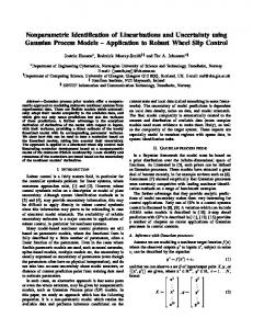
longitude and a latitude. Whenever an individual makes or receives a phone call, the call is routed through a BTS that gives coverage to the cell phone. The geographical area covered by a BTS ranges from less than 1 km2 in dense urban areas to more than 3 km2 in rural areas. For simplicity, we assume that the cell of each BTS tower can be approximated with a 2-dimensional non-overlapping region computed using Voronoi tessellation. Figure 1(a) shows a set of BTSs with the original coverage of each cell, and Figure 1(b) presents its approximated coverage computed using Voronoi. CDR (Call Detail Record) databases are generated when a cell phone connected to the network makes or receives a phone call or uses a service (e.g., SMS, MMS, etc.). In the process, and for invoice purposes, the information regarding the time and the BTS tower where the user was located when the interaction took place is logged, which gives an indication of the geographical position of a cell phone at a given moment in time. Note that no information about the exact position of a user in a cell is known. Also, no information about the location of the cell phone is known or stored if no interaction is taking place. From all the data contained in a CDR, our study uses the encrypted originating number, the encrypted destination number, the time and date of the call, the duration of the call, and the latitude and longitude of the BTS tower used by the originating cell phone number and the destination phone number when the interaction took place. Using the information contained in a CDR database we can characterize the different land uses given to a specific urban area. The geographical areas in which the city is going to be divided will be defined by the Voronoi tessellation of the set of BTSs, and each area will be characterized with the corresponding BTS activity (the signature of the BTS tower). The identification of land uses will be implemented using consensus clustering, which will be introduced in detail in the following section. Our study has been done using CDR data collected from all the BTS towers of the city Madrid during a period of 1 moth, from October 1st 2009 to October 31st 2009. The area covered by the city (and its metropolitan area) is of 400Km2 and is served by 1100 towers that collected over 100 million interactions. In order to preserve privacy, all the information presented is aggregated and original records are encrypted. No demographic data was considered or available for this study. None of the authors of this study participated in the extraction of the data. In order to validate our land use hypothesis, we compare our results against official land use data released by the Department of City Planning of the City of Madrid 1 for the year 2008. Figure 2 depicts the official land uses at a block level in the north-west of the city. The Department of City Planning aggregates the information at a block level and considers eleven main land use types: (1) residential: Apartment Buildings, (2) Residential: Individual homes, (3) Residential: mixed, (4) Industrial, (5) Offices, (6) Commercial, (7) Public infrastructures: public buildings, (8) Public infrastructures: road, (9) Public infrastructures: service areas, (10) sport infrastructures and (11) parks.
4. Activity Signatures from CDR Data We define the activity of a BTS, and by extension of its area of coverage, as the number of calls that are managed by that BTS over a given period of time. The activity associated to each BTS is represented as a matrix vn(δ, τ ), with n∈{1, . . . ,N} the BTS identifier, δ∈Δ = {1, . . . , 31} representing each day of the CDR dataset considered, and τ∈ {1, . . . , 288} representing each one of the 5-minute time slots in which each 24 hour period has been divided. Other values for τ were considered but smaller slots increased the processing time without any relevant improvement, while larger slots produced a linear interpolation effect in the activity signature that affected the quality of the results. The signature Xn of btsn is defined by different aggregations of the information contained in the associated activity matrix vn. Three types of aggregation have are proposed: (1) Total aggregation; (2) WeekdayWeekend aggregation and (3) Daily aggregation. The Total aggregation defines the signature of each BTS as the average value of the activities reported for each time slot τ throughout all days δ. Thus, each element Xn(τ) is computed as: X n ( )
1
1 vn ( , ), 1,...,288 || ||
http://www.madrid.org/cartografia/idem/html/web/index.htm
2
(1)
Nevertheless, human dynamics are very different between weekdays and weekend days [1], and those differences should translate into different BTS activity levels. Considering this fact, the WeekdayWeekend representation aggregates the calling activities reported for each time slot τ for two different types of days: weekdays (Monday through Friday, contained in Ω1) and weekend days (Saturday and Sunday, contained in Ω2). The final signature is represented as the concatenation of both components (represented as +): 1 X n,i ( ) (2) vn ( , ), i {1,2}, {1,...,288} | i | i
X n X n,1 X n,2
(3)
Finally, the Daily aggregation can be considered as an extension of the Weekday-Weekend aggregation, in which each day of the week has its own component. Formally it is computed with Equation (2) but considering Ωday with day={mon, tue,wed, thu, fri, sat, sun}, and Equation (3) concatenates the 7 components. All signatures were normalized before identifying land uses. Figure 3 graphically presents three examples of each one of the aggregation types. Figure 3(a) shows the typical curve for Total aggregation with one peak around 12am and another one at around 7pm. In this particular case, because the 7pm peak has a reduced intensity when compared to the 12am peak, the signal probably represents a commercial land use. Figures 3(b) and 3(c) present the same idea but concatenated 2 times and 7 times respectively representing Daily and Weekday-Weekend aggregations.
5. Consensus Clustering for Land Use Identification In the literature we can find approaches to identify land uses using different clustering techniques, such us spectral clustering [3, 14], k-means [20] or FCM[21]. Nevertheless each technique will introduce a bias that will imply that different techniques cluster the same elements in different clusters. In order to avoid the bias introduced by clustering techniques and to identify well defined land uses we propose the use of Consensus Clustering. Consensus Clustering [22] is based on compiling the results of different clustering methods and on reporting only the elements that are co-clustered together by the set of algorithms considered. The technique is typically applied for microarray analysis in order to avoid inter-clustering method inconsistency. For two given elements, all clustering methods must have allocated them to the same cluster in order for them to be assigned to a consensus cluster. This gives a higher level of confidence to the correct assignment of elements appearing within the same cluster. Consensus clustering is based on an agreement matrix A(n x n), being n the number of elements to be clustered (number of BTS in our context). A is an upper triangular matrix that indicates for each combination of elements the number of agreements among the methods for clustering together the two elements, represented by the row and the column indices. The technique uses the agreement matrix to generate an agreement list that contains all the pairs of elements of the matrix where the value is equal to the total number of clustering methods used, C. Then, starting with an empty set of consensus clusters, the first element is created containing the elements of the first pair of the agreement list. Then, the algorithm iterates for the rest of the elements of the agreement list, where, if one element of the current pair is found in a consensus cluster and the other is not, that element is added to the consensus cluster, otherwise a new consensus cluster is created. After the algorithm has iterated for each pair of elements in the agreement list, it outputs the set of consensus clusters found. Figure 4 presents a description of the algorithm that implements consensus clustering. As a running example lets consider C=3 and 7 elements that have been clustered by each technique as follows: (1) the first clustering technique identified 3 clusters containing each one {1, 2, 3}, {4, 5}, {6, 7}; (2) the second technique identified 4 clusters as follows, {1, 2, 3}, {4, 5}, {6}, {7}; and finally (3) the third technique identified 3 clusters,{1, 2, 3}, {4, 5, 6}, {7}. Running the algorithm we will obtain an AgreementList={{1,2},{2,3},{4,5}}, which will produce two consensus clusters CC={{1,2,3}, {4,5}}. In general, the final number of consensus clusters tends to be higher than the original number of clusters of any of the methods used to obtain the agreement matrix. Note that there is no need that the different clustering methods used actually have identified the same number of clusters. Also, the set of consensus clusters obtained will not necessarily contain all the original elements, because those elements for which the clustering techniques used do not agree will not be included in the final set of consensus clusters. This filtering property of consensus clustering is very useful in our case because it will eliminate elements (i.e.
3
BTS coverage areas) that cannot be grouped in any consensus cluster, which implicitly filter areas that have mixed land use.
6. Clustering for Land Use Identification This section presents the application of K-means, Fuzzy Clustering and Spectral clustering for the identification of land uses, which will then be used when implementing consensus clustering. 6.1 K-means K-means aims to partition n observations into k clusters in which each observation belongs to the cluster with the nearest mean. This technique has been used in similar problems, like the identification of agricultural land uses based on types of vegetation from satellite images [9]. Unsupervised clustering techniques, such as k-means, require the number of clusters to be known beforehand. In this case, the different techniques used to determine an optimum number of clusters are based on identifying the clustering which results in compact and well separated clusters. From the variety of techniques available (Davies-Bouldin index[4], Dunn’s index[5], etc.), we have chosen the validity measure presented in [16] as it is shown to outperform the previous techniques in a variety of applications. In this case, the quality of the partition, measured by the cluster validity index, is given by computing the ratio between the intercluster and intra-cluster distances of the partition for each one of the k values (number of land uses) run. An ideal partition will minimize the intra-cluster distance and maximize the inter-cluster distance; therefore, the best partition will be that which minimizes the proposed measure. Given the nature of the kmeans algorithm, where every cluster is defined by its centroid ci, the intra-cluster and inter-cluster distances are formally defined as: intra-cluster
1 k || X n ci ||2 N i 1 X n Ci
inter-cluster min || ci c j ||2 i j
(4) (5)
where Ci is the set of signatures that belong to the cluster defined by centroid ci. Due to the stochastic nature of k-means we executed the algorithm 500 times for each k and kept the results with better (minimum) validity index values. Table 1 presents the minimum validity index values for the Total, Weekend-Weekday and Daily aggregation with k={3, . . . , 8} when using Euclidean distance. In all cases the best value was obtained when using the Weekday-Weekend aggregation. The clustering validity index values indicate that while the Total aggregation loses information (it has higher values in all cases), the Daily aggregation does not add any extra insight when compared with the Weekday-Weekend representation. Within the Weekday-Weekend representation the top two index values are obtained for k=3 and k=5 respectively. The case k = 3 is obvious as our activity signatures are characterized by bimodal distribution (two peaks) at each 24 hour period. Simplifying the interpretation, with k=3 we observe three differentiated land uses: (1) when the first peak is higher than the second one, which will probably indicate an area with commercial and/or industrial activity; (2) when the second peak is higher than the fist peak (a residential area) and (3) when the two peaks have the same height (a mixed used area). Nevertheless, we are interested in identifying a variety of land uses apart from the obvious ones identified by k = 3. The second case, k = 5 is much more interesting, as intermediate land uses are found. With this fact in mind, we consider that the best validity index is obtained a Weekday-Weekend aggregation and k = 5. In this case from the approximately 1100 areas of coverage, 11% were included in cluster 1, 15% in cluster 2, 5% cluster 3, 7% in cluster 4 and 62% in cluster 5. The class representatives of each cluster are presented in Figure 5. An analysis of these signatures allows to hypothesize about each land use: • Cluster #1 (Figure 5(a)): This cluster is characterized by the fact that the activity takes place mainly during weekdays, especially in working hours, and weekend activity is very reduced. During weekdays the activity is heavily focused between 10AM and 14PM and another peak of activity between 16:00 and 19:00 hours. This cluster shows a work related activity pattern and the hypothesis is that the BTS coverage areas included in this cluster are used as industrial parks and/or office areas. The geographical representation of the cluster is presented in Figure 7(a). For future reference this cluster will be named as Offices&Industrial.
4
• Cluster #2 (Figure 5(b)): The second cluster probably represents a hybrid land use. During weekdays there is activity during commercial hours, with two peaks of similar normalized intensity at around 12AM and 19PM. There is a relevant weekend activity although of less intensity. This behavior could be considered Commercial. The lesser intensity of both peaks during weekends is probably caused because commerce in Spain is generally closed on Sundays. • Cluster #3(Figure 5(c)): The third cluster has one element that characterizes its land use: during weekends there is a strong activity between 0AM and 5AM, indicating nightlife environments. The land use derived from this behavior is Nightlife areas: restaurants, bars, etc. • Cluster #4 (Figure 5(d)): This class representative shows that activity during weekends is more than twice that of weekdays, and that this activity is focused between 12PM and 5PM. The geographical representation of this cluster is presented in Figure 7(b). Considering all the information, this land use probably characterizes weekend Leisure activities. • Cluster #5 (Figure 5(e)): This signature shows that activity during weekdays and weekends is of the same magnitude. During weekdays, the second peak of activity is of higher magnitude than the morning peak, while during weekends both peaks have the same magnitude. These characteristics imply Residential areas, where individuals come back after work and stay during weekends. The main limitation of this approach is that the land uses identified are constructed using all the original BTSs, which as a results creates signatures that inherently represent combinations of different behaviors. Cluster #2 is a good example of this fact. Ideally signatures should be defined by the core elements of each land use, without considering elements that are distant from the class representative. In any case, by definition, k-means does have such a mechanism. 6.2 Fuzzy Clustering for Land Use Identification Fuzzy c-means (FCM) clustering [2] assigns to each element a degree of belonging to each cluster. The algorithm attempts to partition a finite collection of elements X={x1,…,xn} into a collection of c fuzzy clusters. Given a finite set of data, the algorithm returns a list of c cluster centres C={c1,…,cc} and a partition matrix U=ui,j є (0,1) ,i=1,…n, j=1,…,c, where each element of the matrix tells the degree to which xi belongs to cluster cj. Fuzzy c-means needs as input the number of clusters and the fuzziness coefficient m. The fuzzifier m (1< m < ∞) determines the level of cluster fuzziness, where a large value of m results in fuzzier clusters. In the limit, m=1 and the memberships converge to 0 or 1, i.e. a crisp partition. This technique has also been used in similar problems, like the classification of sub urban land using remotely sensed imagery [26]. We have used FCM to cluster the BTS signatures and obtain the class representatives that define land uses. In order to find the optimal number of clusters we have used subtractive clustering [5]. This method assumes every item in the dataset might be a cluster center and assigns a potential value to them. The method iteratively picks the item with the highest potential, selects it as a cluster center, and decreases the potential of the surrounding items that are situated within a radius of influence rinf. Low rinf values produce a large number of small clusters, while the opposite happens with high rinf values. Common values for rinf are in the range (0.25, 0.45). Figure 6(a) shows the number of clusters for each value in the mentioned interval with 0.01 increments. It can be observed that the curve decreases drastically in rinf = 0.4, and stabilizes in 5 clusters (Fig. 6(b)). We used the method presented in [7] to estimate m, finding an optimum value of m = 1.2. The land use representatives obtained after running fuzzy c-means with 5 clusters and m = 1.2 are fairly similar to the ones obtained by k-means and presented in Figure 5, with some small differences in the level of activity of the peaks and the geographical representation of the clusters, but the same hypothesis about land use are valid. Considering the characteristics of FCM, each area of coverage was assigned to the cluster that had the highest degree ui,j. In that case 14% of BTSs were included in cluster 1, 11% in cluster 2, 12% cluster 3, 9% in cluster 4 and 54% in cluster 5. As examples, Figure 8(a) and Figure 8(b) present the geographical representation of Cluster #2 and Cluster #5 when using FCM. 6.3 Spectral Clustering Spectral clustering [27] treats the data clustering problem as a graph partitioning problem without making any assumptions about the shape of the data clusters. The technique has four main stages: (1) construct the similarity matrix D with the data (which implicitly also builds a graph based on similarities); (2)
5
compute the associated Laplacian matrix L and obtain its eigenvalues and eigenvectors; (3) use the eigenvectors to match each original data point to a lower-dimensional representation and (4) cluster the data points in the reduced dimension. The main characteristic of the technique is to use the eigenvalues (i.e. the spectrum) of the similarity matrix to produce a dimensionality reduction. Spectral clustering also needs to define before hand the number of clusters k. Although any techniques used in clustering can be potentially used to identify the optimum number of clusters, the use of eigenvalues is especially useful due to the nature of the algorithm. The eigengap heuristic [13] identifies k as the point where the largest drop in the magnitude of the ordered eigenvalues happens We used Spectral Clustering to cluster the BTS signatures and obtain the class representatives that define land uses. We generated the similarity matrix (D) using the cosine similarity between each pair of activity vectors Xi and Xj: s (i , j )
Xi X j Xi X j
(6)
The eigengap heuristic identified k=6 as the optimum number of clusters. As a result spectral clustering identified 6 land uses with their respective cluster representatives. The land use representatives obtained in this case are similar to the ones obtained for Cluster #1, #2, #3 and #5 when using k-means (Figure 5), although there are differences when the graphical representation of the clusters is considered. The extra cluster identified by spectral clustering basically implied that Cluster #4 has been divided in two different land uses, whose activity signature is fairly similar to the ones presented in Figure 13(a) and Figure 13(b). For homogeneity purposes we call these two new clusters Cluster #4.1 and Cluster #4.2. An analysis of these signatures allows to hypothesize about each land use: • Cluster #4.1: Spectral cluster 4.1 has a very similar signature to the Cluster #4 produced by kmeans/FCM (Figure 5(d)), but in this case, the weekday activity, has been drastically reduced when compared to the K-means/FCM signature. The land use is probably related with weekend leisure activities. • Cluster #4.2: Spectral cluster #4.2 describes land uses that are more active during weekends than weekdays, and where the traditional two peaks behavior is not as strong as it typically is. Although in this case the signature activity is not enough to hypothesize a land use, the graphical representation of the BTS shows that the area covered mainly includes transportation hubs, such as the 4 terminals of the airport, the train station and the bus station. As a result, we hypothesize that the cluster represents transportation hubs land use. When using spectral clustering, 16% of BTSs were included in cluster 1, 13% in cluster 2, 8% cluster 3, 6% in cluster 4.1, 4% in cluster 4.2 and 53% in cluster 5.
6.4 Comparative Analysis & Validation In order to compare the clusters obtain by each one of the previous techniques, first we will measure the similarity of the data partitions and after that we will validate each technique comparing it with the real land use data obtained from the Department of City Planning. 6.4.1 Cluster Similarities Differences within clustering techniques are typical, and they have motivated the development of techniques that compare the level of agreement between two classifiers. These techniques can also be presented as a way of assessing the consistency of a partition. A simple method for comparing two data partitions is the Kappa metric [23, 24]. This metric rates the agreement between the classification decisions made by two observers. The metric has a value in the range (-1, +1), where -1 indicates that there is no concordance between the observers, and +1 indicates total concordance. From a clustering perspective, a high kappa value would indicate that the two arrangements are similar, while a low value would indicate that they are dissimilar. The kappa value between k-means and Fuzzy Clustering is 0.59, between k-means and Spectral clustering 0.48, and between Fuzzy clustering and spectral clustering 0.51. The three values indicate a moderate agreement between the techniques. This result shows that the partitions created are not very consistent. This is in part caused by the fact that each technique has a bias
6
that deeply affects its classification. In order to identify reliable land uses, we need to use a technique that counteracts the bias of the techniques. 6.4.2 Land Use Validation In this section we will validate each technique by comparing its output with the land use information available at the Department of City Planning. Visually speaking, we want to understand the percentage of overlapping that exists between the CDR land uses we have identified with each clustering technique and the official land use areas declared by the Department of City Planning. Such overlapping will give us an understanding of the accuracy that CDR activity achieves in identifying land uses i.e., the larger the overlapping areas, the more accurate CDR activity is for modelling land use. It is important to highlight that the percentage of overlapping is an approximate measure to validate land use identification given that both maps have different granularities: CDR maps represent land segment clusters based on Voronoi, whereas the Madrid information contains data at a block level. In order to analyze overlapping areas, we used GIS software [6] that allowed to evaluate the overlapping between the shapefiles of two given regions. In our case, one shapefile will represent the land use cluster we have obtained and the other one an official land use. Tables 2, 3 and 4 show the percentages of overlap between the official land uses (rows) and our land use hypothesis (columns). Specifically, each element (i, j) in the table represents the percentage of the official land use i that is covered by one of our CDR land use clusters j. In the case of Table 2 and Table 3, that present the results when using K-means and FCM respectively, for comparison purposes, we grouped the official land uses as: (1) Residential (the three levels defined), (2) Offices & Industrial & Public Buildings & Service Areas, (3) Commercial and (4) Parks and Sport Infrastructures. The official land use Roads was not considered. So, in this case, i={Residential, Offices & Industrial & Public Infrastructures, Commercial, Parks} and j={Offices, Residential, Commercial, Nightlife, Leisure}. In Table 4, when considering the results provided by spectral clustering, due to the extra cluster identified as transportation hubs, we considered as official uses i={Residential, Offices & Industrial, Public Infrastructures, Commercial, Parks} and our CDR land uses as j={Offices, Residential, Commercial, Nightlife, Leisure, Transport}. Note that the overlap, due to the different granularity of the elements being compared, and the fact that the official land use Road is not considered, does not necessarily adds up to 100%. Table 2 presents the overlap between the official land uses and the CDR land uses when using K-means. We observe that the official Offices&Industrial land use is identified with coverage of 63% by the CDR Offices land use. Nevertheless there is also a relevant overlap of 21% with Commercial land use. The official Residential land use is also well identified by the CDR Residential land use, with coverage of 61%, although there is also a relevant coverage with Commercial and Nightlife CDR land uses. Commercial land use has an overlap of 57% while Parks has the strongest overlap with 78%. The CDR land use of Nightlife can not be validates as it is not considered by the Department of City Planning, and gets mixed basically with the official Residential land use, which indicates a mixture of those land uses. Table 3 presents the overlap between the official land uses and the CDR land uses when using FCM. In general the same results and observations presented for K-means, are also true in this case, with overlapping values of the same magnitude in both cases. Table 4 presents the overlap between the official land uses and the CDR land uses when using Spectral Clustering. When compared to the two previous techniques, there is an improvement in the overlap, which in general can be attributed, to the variability of cluster shapes that spectral clustering can identify. Also, the special case of Transport CDR land use, has an overlap of 33% with public infrastructures. Transportation hubs are included in the Public Infrastructure official land use, but it is obviously not the only one, that is the reason for the low overlap. If we consider the inverse relation, i.e. the percentage of Transport CDR land use included in the official Public Infrastructures land use, the overlap is 88%, which indicates how all the areas identified are considered a Public Infrastructure. In general we can conclude that CDR land uses are validated with Official land uses, especially when considering the results provided by spectral clustering. In general the level of overlap is in the range 60%70% which is caused mainly by (1) the fact that that CDR identifies the real land use while the department of city planning has the planned use, which could change over time, (2) the fact that the granularity of both land uses maps is quite different, and (3) the fact that in an urban environment the same geographical area can have a variety of land uses which the approach of the Department of City Planning does not consider. This indicates that using a Consensus clustering approach, with its capability of filtering elements, can potentially increase our land use detection.
7
7. Land Use Analysis with Consensus Clustering The kappa metrics and the validation results of the previous section indicate that there are divergences between the land uses identified and the clusters produced by each technique. In this context, consensus clustering can be relevant due to its capability of limiting the bias of each technique. Considering that the area selected is covered by 1,100 cells and using results from three different clustering algorithms, the Agreement Matrix A was of dimension 1100x1100, with C=3. After applying the algorithm, we obtained eleven clusters with 39% of the BTSs being filtered, i.e. the consensus clustering algorithm did not assign them to any of the final clusters. Figure 9 through Figure 18 presents the eleven signatures of the consensus clusters identified and their corresponding geographical representation within Madrid. Generally speaking, Madrid is contained inside two concentric ring roads (M-30 and M-40). The area inside the M-30 (the smaller ring) contains the city center as well as the main business, tourist and commercial areas, all of them mixed with residential areas. The main avenue is Paseo de la Castellana which is the main north-south axis of the city and the business area. The area comprised between the M30 and M-40 contains mainly residential districts and industrial parks. An analysis of the signatures and their geographical distribution allows to hypothesize about the land uses: • Consensus Cluster #1 (Figure 9(a)) and Consensus Cluster #2(Figure 9(b)): The signatures of these clusters are similar to one presented in Figure 5(a) which represented Offices/Industrial parks. The main differences is that in the case of Consensus Cluster #1 (CC #1) the activity level during weekends is almost doubled when compared to Figure 5(a), while Consensus Cluster #2 (CC#2) the activity during weekends is almost non existent. Figure 10(a) and 10(b) present the geographical representation of CC #1 and CC #2 respectively. Considering these representations, it can be observed that while CC #1 covers Offices within the city (the areas around the Paseo de la Castellana, AZCA and public buildings such as the City Hall and the Congress), CC #2 covers Industrial parks outside the M-30, which explains the difference in activity during weekends. As a result we hypothesize that while CC #1 represent Offices, CC #2 represents industrial parks. These two consensus clusters are a good example of the advantages of using consensus clustering: the effect of co-clustering is the identification of land uses that were originally aggregated in one or more clusters. • Consensus Cluster #3 & Consensus Cluster #4 (Figure 11(a) and 11(b)): These two clusters are related to Cluster #3 presented in Figure 5(c). Both CC #2 and CC #3 are characterized by a peak of activity at night which uniquely differentiates them from the rest of the clusters. While CC #2 basically represents the same behavior as Figure 5(c), i.e. night activity areas during weekends, CC #3 shows activity early in the morning (starting at 4am) both during weekdays and weekends, which motivated that they were clustered together when using k-means/FCM/Spectral clustering. Considering the geographical representations of CC #3 and CC #4 presented in Figure 12(a) and Figure 12(b) respectively we can observe that CC #2 covers the main nightlife areas of the city: Gran Via, Bilbao, Moncloa and Alonso Martinez. Part of the Campus where the university dorms are located is also included in this cluster. CC #3 is very limited in size (only 6 BTS towers) and actually corresponds to MercaMadrid, the wholesale food market of the city (one of the biggest food markets in Europe), whose activity takes place during early morning, including weekends. No other geographical areas are included in this land use. Both consensus clusters are related to nigh activity, but while CC #3 probably represents nightlife leisure areas, CC #3 represents early morning commercial activities. • Consensus Cluster #5 & Consensus Cluster #6 (Figure 13(a) and 13(b)): These two consensus clusters are related with Cluster #4 presented in Figure 5(d) that represented weekend leisure activities. Their main characteristic is that there is more activity during weekends than during weekdays. Nevertheless while CC #5 has almost no activity during weekdays, CC #6 has a relevant activity during weekdays showing the typical bimodal distribution. Considering the geographical representations of CC #5 and CC #6 presented in Figure 14(a) and Figure 14(b) respectively, we can observe that the areas covered by CC #5 include the main parks and recreational areas of the city, like Casa de Campo and El Pardo, golf clubs (marked as GC) and the Horse Racing Track (marked as H). Within the city, El Prado Museum (including the botanical gardens) and the flea market (which happens Sunday mornings) are included in this land use. Regarding CC #6 it covers the main transportation hubs of the city: all the terminals of Barajas International Airport, the Bus Station and Atocha Train Station, that serves as a hub for high speed trains (Chamartin train station in the north of the city is the only hub not included in this cluster).
8
Again, another good example of finding clusters previously aggregated thanks to the co-clustering effect of consensus clustering • Consensus Cluster #7 and Consensus Cluster #8 (Figure 15(a) and 15(b)): Both consensus clusters have an activity signature similar to Cluster #5 of Figure 5(e) which indicates that they probably represent residential land use. Their differences are mainly in weekend activity which is lower in CC #8 when compared to CC #7. If the geographical representation is considered, Figures 16(a) and 16(b) for CC #7 and CC #8 respectively, it can be observed that CC #7 accounts for approximately 40% of the geographical area. It is highly correlated with high-density residential areas (high rises), mainly in the south and east of the city. The geographical representation of CC #8 covers residential area of low and mid density (individual houses and low rises), mainly located in the west and north of the city. This distribution is typical in Madrid, where affluent areas are located west and north of the city. In any case, although downtown also includes a large number of residential areas, none of the residential clusters identified are present in that area. The main reason for this fact is that consensus clustering filters out those areas because in general they concentrate a variety of activities and as a result those BTSs are not co-clustered together. • Consensus Cluster #9 & Consensus Cluster #10 & Consensus Cluster #11 (Figures 17(a), 17(b) and 17(c)): These consensus clusters are related to Cluster #2 of Figure 5(b) that represented commercial activity. The three cases identified by consensus clustering identify different levels of commercial activity. Consensus Cluster #10 (Figure 17(b)) represents basically the same behavior as Cluster #2 (Figure 5(b)): commercial activities take place basically in the morning during weekdays, and a reduced activity during weekends due to the fact that, in general, commerce is typically close on Sundays. The geographical representation of CC #10 (presented in Figure 17(b)) focus mainly around the main commercial districts of the city: Salamanca, Chamartin and Chamberi. These districts have a strong commercial activity, but are also densely populated residential areas. Commerce in these neighborhoods closes on Sunday which motivates the reduction of activity during weekends. The other two consensus clusters show two deviations from that main use: (1) consensus cluster #9 (Figure 17(a)) shows commercial areas that have the same activity during weekdays and weekends, which should correspond to special parts of the city that are allowed to open on Sundays; and (2) consensus cluster #11 (Figure 17(c)) shows commercial areas that have more activity during weekdays than weekends, which should represent weekend commercial areas. The geographical representation of CC #9 is presented in Figure 18(a), and it shows that the geographical areas included in this land use are around Puerta del Sol, Plaza Mayor and Plaza de Santa Ana, the main touristic areas of the city. Commerce opens during weekends in these areas. Last, Figure 18(c) presents the geographical representation of CC #11, which covers the main commercial axis of Madrid (Callao-Preciados) and its surroundings. Commerce in this area opens both weekends and weekdays. We can observe how the consensus clusters identified benefit from the filtering and co-clustering imposed by the technique: (1) the clusters identified have land uses obtained only with coverage areas that have a well defined behavior and (2) the co-clustering allows to identify intermediate land uses that could not be identified with traditional techniques. 7.1 Validation of Consensus Land Uses In this section we are going to use the information provided by the Department of City Planning (DCP) to validate to which extent the land uses identified by consensus clustering are similar to the ones defined by DCP. Nevertheless, when using this information for validation purposses, two elements have to be considered: (1) the information is mainly regarding how land use is planned (urban zoning) not on the actual use of the land, which is not necessarily the same; and (2) urban planning focuses mainly on defining residential and industrial areas, not the variety of uses we have discovered. In order to validate the consensus clusters we will consider the following official land uses, grouping some of them: (1) Residential: Apartment buildings, (2) Residential: individual homes and mixed, (3) Industrial, (4) Offices & Public infrastructures: public buildings, (5) Commercial, (6) Public infrastructures: service areas and (7) parks and sport infrastructures. Regarding the land uses identified by consensus clustering, we will group CC #9, CC #10 and CC #11 into one cluster, as the official land use just considers commercial areas, not the variety we have identified. Also, when validating the land uses we have to consider that consensus cluster has filtered almost 40% of the BTS areas, i.e. 40% of the terrain has not been classified. As a result, the validation is implemented by considering for each
9
consensus land use the percentage that is included in each official land use (which covers all the terrain). Table 5 shows these values, where each element (i, j) in the table represents the percentage of the consensus land use i that is included in each one of the official land uses considered j. Note that each row does not add up exactly to 100% because: (1) the granularity of the consensus and official land use classification is very different (Voronoi tessellation vs. city blocks) and (2) the official land use Roads has not been considered. We can observe that consensus clustering identifies more land uses than traditional clustering approaches (eleven compared to five or six), and that for the land uses that are common with traditional clustering techniques, there is an improvement in the level of overlapping. Focussing on the results presented in Table 5, some of the consensus land uses have a high correlation with the official land use, such as Offices, Residential-High, Residential-Low and Leisure, with correlation in all cases above 70%. In the case of MercaMadrid and Hubs, the coverage is above 80% with the official land use Public Infrastructures, because that is what they are considered by the DCP. As in the previous approaches, Nightlife has a high correlation with Residential-High, but there is no official land use to validate it. The three types of consensus commercial activities have a correlation of 65% with the official land use, but it is not possible to validate each one of them individually. The exception to this improved results is the Industrial land use, with a value of just 52%, highlighting the difficulty of identifying Industrial land uses in urban environment using cell phone activity, probably mainly due to the interferences introduced by roads (in any case, this land use was not uniquely identified by any of the previous clustering techniques). In order to compare the results of Consensus Clustering with FCM, K-means and Spectral Clustering from the clustering perspective, we calculated the compacity of the clusters obtained using the validity index presented in equations (4) and (5). K-means index, for the 5 clusters considered was 0.54, 0.49 was obtained for FCM and 0.42 for Spectral clustering. The index obtained for Consensus Clustering is 0.31 which is a considerable improvement when compared to traditional techniques. This improvement is mainly caused by the ability of consensus clustering to filter BTSs that do not show a well defined behavior and by the capability of finding smaller and better defined clusters.
8. Conclusions and Future Work We have presented a data mining approach to the problem of identifying land uses in an urban landscape using the information collected from cell phone networks. Our approach, which uses consensus clustering, is designed to overcome the bias of traditional clustering techniques in order to identify the BTS activity signatures that are key in defining land uses. We have validated the results obtained with official land use data obtained from the Department of City Planning. This data has some limitations, as it is obtained with traditional techniques, but gives a baseline to compare the different approaches. Our results show the improvement that using consensus clustering implies compared with traditional clustering techniques: there is an increase in the number of land uses identified and the correlation values used for validation are higher. The use of data mining techniques applied over sensor data for urban analysis is a big improvement when compared to traditional approaches that are based on questionnaires/surveys. These traditional approaches for capturing data face cost and time limitations. Our solution overcomes these limitations and brings new advantages like the capability of tracing land use evolution over time or the ability to focus the study for a particular social background (elders, tourists, socio-economic levels, etc.) by just considering the information originating from those groups. In any case, our approach is not intended to substitute traditional urban analysis approaches but to complement and improve them. For future work we plan to use our technique to implement a tool designed to evaluate the degree to which the urban zoning planned by a city hall is actually being followed. The identification of the differences can then be used to implement a better planning of public resources. For example, nightlife areas are difficult to track, as they change frequently and are important because they require resources such as police or cleaning services. The availability of a tool that automatically identifies and track those areas over time will facilitate optimum planning of public resources.
10
References [1] I. Benenson and E. Hatna, Human choice behavior makes city dynamics robust and, thus, predictable, GeoComputation (2003). [2] J.C. Bezdek and R. Ehrlich, FCM: The fuzzy c-means clustering algorithm, Computers & Geosciences 10(2-3) (1984) 191-203. [3] J. Cranshaw, R. Schwartz, J. Hong & N. Sadeh, The livehoods project: Utilizing social media to understand the dynamics of a city, ICWSM'12 (2012) [4] D.L. Davies and D.W. Bouldin, A cluster separation measure, IEEE Trans. Pattern Anal. Machine Intell. Vol. 1 (1979) 224-227. [5] J.C. Dunn, A fuzzy relative of the ISODATA process and its use in detecting compact well-separated clusters, Journal of Cybernetics, vol. 3 (1973) 32-57. [6] ESRI, http://www.esri.com/software/arcgis/index.html [7] E. Frias-Martinez, G. Williamson, V. Frias-Martinez, An Agent-Based Model of Epidemic Spread using Human Mobility and Social Network Information, in: The 3rd IEEE Int. Conf. on Social Computing- SocialCom (2011). [8] T. Fujisaka, R. Lee, and K. Sumiya, Exploring urban characteristics using movement history of mass mobile microbloggers, in: Proc. of the 11th Workshop on Mobile Computing Systems & Applications (2010) 13–18. [9] K.S. Han, J.L. Champeaux and J.L. Roujean, A land cover classification product over France at 1 km resolution using SPOT4/VEGETATION data, Remote Sensing of Environment 92(1) (2004) 52-66. [10] T. Horanont and R. Shibasaki, Evolution of urban activities and land use classification through mobile phone and gis analysis, In: 11th Int. Conf. on Computers in Urban Planning and Urban Management CUPUM (2009). [11] S. Kinsella, V. Murdock, and N. Oare, I am eating a sandwich in Glasgow: modeling locations with tweets, in: Proc. of the 3rd Workshop on Search and Mining User-generated Contents (2011). [12] L. Liao, D. Paterson, D. Fox, and H. Kautz, Learning an inferring transportation routines, Artificial Intelligence, vol. 171(5-6) (2007) 311-331. [13] U. Luxburg, A tutorial on spectral clustering, Technical Report 149, Max Planck Institute for Biological Cybernetics, 2006 [14] A. Noulas, S. Scellato, C. Mascolo, and M. Pontil, Exploiting semantic annotations for clustering geographic areas and users in location-based social networks, in: 3rd Workshop Social Mobile Web (SMW 2011)- Colocated with ICWSM 2011. [15] C. Ratti, R.M. Pulselli, S. Williams and D. Frenchman, Mobile landscapes: using location data from cell phones for urban analysis, Environment and Planning B: Planning and Design 33(5) (2006) 727–748. [16] S. Ray and R. H. Turi, Determination of number of clusters in k-means clustering and application in colour image segmentation, in: Proc. 4th int. conf. on advances in pattern recognition and digital techniques - ICAPRDT (1999) 137-143. [17] J. Reades, F. Calabrese, A. Sevtsuk and C. Ratti, Cellular census: Explorations in urban data collection, IEEE Pervasive Computing 6(3) (2007) 30–38. [18] J. Reades, F. Calabrese, C. Ratti, Eigenplaces: analysing cities using the space time structure of the mobile phone network, Environment and Planning B: Planning and Design 36(5) (2009) 824–836. [19] J. Schiller and A. Voisard, Location-Based Services. Morgan Kaufmann, 2004. [20] V. Soto and E. Frias-Martinez, Automated Land Use Identification using Call Detail Records, in: 3rd ACM Int. Workshop on Hot Topics in Planet-Scale Measurement, in conjunction with ACM MobiSys2011 (2011). [21] V. Soto and E. Frias-Martinez, Robust Land Use Characterization of Urban Landscapes using Cell Phone Data, in Workshop on Pervasive Urban Applications in conjunction with 9th Int. Conf. on Pervasive Computing (2011). [22] S. Swift, A. Tucker, V. Vinciotti, N. Marin, C. Orengo, X. Liu, P. Kellam, Consensus Clustering and Functional interpretation of gene-expression data, Genome Biology 5 (11) (2004) R94. [23] J.S. Uebersax, Diversity of decision-making models and the measurement of interrater agreement, Psycological Bulletin 101 (1987) 140-146. [24] C. Valiquette, A. Lesage, M. Cyr and J. Toupin, Computing Cohen’s kappa coefficients using SPSS MATRIX, Behavioral Research Methods, Instruments and Computers 26 (1994) 60-61. [25] S. Wakamiya, R. Lee, and K. Sumiya, Urban area characterization based on semantics of crowd activities in twitter, in: C. Claramunt, S. Levashkin, and M. Bertolotto, editors, GeoSpatial Semantics, vol. 6631 of Lecture Notes in Computer Science (2011) 108–123. [26] J. Zhang and G.M. Foody, Fully-fuzzy supervised classification of sub-urban land cover from remotely sensed imagery: statistical and artificial neural network approaches, International Journal of Remote Sensing 22(4) (2001) 615-628. [27] J. Shi and J. Malik, Normalized cuts and image segmentation, Proceedings of the Conference on Computer Vision and Pattern Recognition, 1997.
11
(left)
(right)
Figure 1: (left) Example of a set of BTS and their coverage and (right) approximated coverage obtained applying Voronoi Tessellation.
Figure 2: Example of official land use released by the Department of City Planning for 2008.
12
(a)
(b)
(c)
Figure 3: Example of (a) Total, (b) Daily and (c) Weekend-Weekday aggregation.
Figure 4: Consensus Clustering Algorithm with A(n x n) the agreement matrix and C the number of clustering techniques used.
Weekday-Weekend Daily Total
3 0.2 0.26 0.3
Number of Clusters 4 5 6 7 0.6 0.54 0.6 0.68 0.6 0.59 0.69 0.7 0.84 0.8 0.81 0.84
8 0.67 0.75 0.85
Table 1: Cluster validity index when using K-means with Euclidean distance, each aggregation type (WeekdayWeekend, Daily & Total) and k={3,…,8}.
13
Figure 5: From left to right and top to bottom, class representatives of cluster #1 through cluster # 5 of the land uses identified by k-means when using the Weekday-Weekend aggregation and Euclidean distance.
(a) (b) Figure 6: (a) Evolution of rinf vs. number of centroids in interval [0.25,0.45], and (b) in [0.4,0.45].
14
(b)
(a)
Figure 7: (a) Geographical representation of Cluster #1 (Office Areas) obtained with K-means and (b) Geographical representation of Cluster #4 (Leisure Activities) obtained with K-means.
(a)
(b)
Figure 8: (a) Geographical representation of cluster #2 (Commercial Areas) obtained with FCM and (b) Geographical representation of cluster #5 (Residential Areas) obtained with FCM.
15
Official Land Use
K-Means Land Use Residential
Offices
Commercial
Nightlife
Leisure
Residential
61%
6%
12%
15%
4%
Offices & Industrial & PI
9%
63%
21%
1%
2%
Commercial
16%
9%
57%
4%
8%
Parks
4%
6%
7%
2%
78%
Table 2. Percentage of overlap between official land use and K-means land use.
Official Land Use
FCM Land Use Residential
Offices
Commercial
Nightlife
Leisure
Residential
63%
7%
10%
12%
2%
Offices & Industrial & PI
6%
66%
15%
8%
1%
Commercial
15%
13%
52%
7%
9%
Parks
13%
1%
2%
3%
77%
Table 3. Percentage of overlap between official land use and FCM land use.
Spectral Land Use Official Land Use Residential
Offices
Commercial
Nightlife
Leisure
Transport
Residential
69%
4%
10%
12%
2%
1%
Offices & Industrial
14%
70%
11%
1%
1%
0%
Public Infrastructures
21%
24%
11%
2%
5%
33%
Commercial
15%
10%
63%
4%
2%
1%
Parks
6%
3%
2%
4%
81%
0%
Table 4. Percentage of overlap between official land use and Spectral land use.
16
Figure 9: Class representatives of (a) consensus cluster #1 (Office Areas) and (b) consensus cluster #2 (Industrial Areas).
(a)
(b)
Figure 10: (a) Geographical representation of Consensus Cluster #1 (Office Areas) and (b) Consensus Cluster #2 (Industrial areas).
17
Figure 11: Class representatives of (a) consensus cluster #3 (Nightlife) and (b) consensus cluster #4 (Wholesale Market).
(a)
(b)
Figure 12: (a) Geographical representation of Consensus Cluster #3 (Nightlife activities) and (b) Consensus Cluster #4 (Wholesale Market).
18
Figure 13: Class representatives of (a) consensus cluster #5 (Leisure activities) and (b) consensus cluster #6 (Transportation Hubs).
(a)
(b)
Figure 14: (a) Geographical representation of Consensus Cluster #5 (Leisure Activities) and (b) Consensus Cluster #6 (Transportation Hubs).
19
Figure 15: Class representatives of (a) consensus cluster #7 (High density residential areas) and (b) consensus cluster #8 (low-medium density residential areas).
(b)
(a)
Figure 16: (a) Geographical representation of Consensus Cluster #7 (High density Residential areas) and (b) Consensus Cluster #8 (Low-Medium density Residential Areas).
20
Figure 17: Class representatives of (a) consensus cluster #9 (Tourist Commercial Areas), (b) consensus cluster #10 (Regular Commercial Areas) and (c) consensus cluster #11 (Weekend Commercial Areas).
(a)
(b)
(c) Figure 19: From left to right and top to bottom, geographical representation of (a) consensus cluster #9 (Tourist Commercial Areas); (c) consensus cluster #10 (Regular Commercial Areas) and (d) consensus cluster #11 (Weekend Commercial Areas).
21
Official Land Use Consensus Cluster Land Use
Residential - High
Residential – Med& Low
Industrial
Offices
Commercial
Public Infrastructures
Parks
CC #1(Offices)
10%
0%
9%
73%
3%
0%
0%
CC #2 (Industrial)
4%
5%
52%
19%
8%
4%
1% 2%
CC #3 (Nightlife)
44%
8%
6%
21%
13%
2%
CC #4 (MercaMadrid)
0%
0%
0%
0%
0%
86%
9%
CC #5 (Leisure)
1%
6%
3%
0%
0%
0%
85%
CC #6 (Hubs)
1%
0%
5%
0%
0%
82%
7%
CC #7 (ResidentialHigh)
72%
9%
2%
3%
8%
0%
1%
CC #8 (Residential – Low)
9%
77%
0%
3%
0%
0%
6%
CC #9 & CC #10 & CC #11 (Commercial)
21%
0%
0%
7%
65%
1%
1%
Table 5. Percentage of overlap between consensus land use and official land use.
22