Nonparametric Identification Assuming Two Noise

828

IEEE TRANSACTIONS ON INSTRUMENTATION AND MEASUREMENT, VOL. 47, NO. 4, AUGUST 1998

Nonparametric Identification Assuming Two Noise Sources: A Deconvolution Approach Tam´as Dab´oczi

Abstract— Nonparametric identification of linear systems is investigated in this paper. Nonparametric identification is the estimation of the time record of the impulse response of the system. It is a deconvolution problem, i.e., inverse operation of the convolution of the impulse response and the excitation signal. The problem is ill posed, i.e., deconvolution amplifies the measurement noise to a great extent. The noise has to be suppressed with the price of a bias in the estimate. A tradeoff has to be found between the noisy and biased estimates. Because of the need for repeatability and to reduce the subjectivity, the level of noise reduction has to be set algorithmically. This paper introduces a method that optimizes the parameter(s) of deconvolution filters and, thus, controls the level of noise reduction. The proposed method assumes observation noise sources for both the measurement of the excitation signal and the system output. Index Terms—Deconvolutions, identification, inverse problem, nonparametric identification, signal reconstruction, signal restoration.

I. INTRODUCTION

to large deviations in the estimation [1], [2]. In other words, the deconvolution process amplifies the measurement noise. This noise has to be suppressed [3]. However, suppression of the noise leads to bias of the useful signal. A tradeoff has to be found in the level of the noise reduction to keep a balance between the variance and the bias. The level of noise reduction is usually controlled with one or a few parameters of the deconvolution filter. In order to ensure repeatability and reduce the level of subjectivity, the level of noise reduction should be determined algorithmically, which is the aim of this paper. It will be shown that the extension of a previous work [4], [13] improves the capabilities of the algorithm significantly, by taking both input and output observation noises into account. The results can be used also for signal reconstruction problems. In this case, the second noise source, in addition to the output noise, is the uncertainty of the estimate of the transfer function.

I

DENTIFICATION of linear systems is the estimation of some characteristic function of the system (e.g., impulse response, transfer function, step response etc.). Parametric identification consists of two steps. First, an appropriate model should be set up for the structure of the system; then the parameters of the system have to be estimated. The result of nonparametric methods is the time or other domain waveform of a characteristic function of the system (impulse response, transfer function etc.), without any explicit information about the structure of the system. As a consequence, nonparametric identification is preferred if the structural information is lacking. The output signal of the investigated system is the convolution of the excitation signal with the impulse response. Thus, nonparametric identification is a deconvolution problem (inverse operation of convolution). The problem is ill-posed, which means that a small uncertainty in the measurement leads Manuscript received May 18, 1997; revised December 21, 1998. This work was supported by the Hungarian Fund for Scientific Research under Grants OTKA F16457, F26136, and OTKA T021 003. This work was also supported in part by the National Institute of Standards and Technology (NIST), Gaithersburg, MD, under Grant 43NANB614 883 and by the Electronic Instrumentation and Metrology Group (led by B. A. Bell). The author is with the Department of Measurement and Information Systems, Technical University of Budapest, Budapest, H-1521 Hungary. Publisher Item Identifier S 0018-9456(98)09943-4.

II. PREVIOUS WORKS One of the earliest results is reported in [5], developed by Guillaume and Nahman in the early 1980’s. The estimated impulse response is calculated in the frequency domain. The measured signal is transformed into the discrete Fourier transform (DFT) domain, filtered, and transformed to the discrete time domain. The originally real signal becomes complex because of the computational errors. The standard deviation of the imaginary part of the estimated signal is minimized to obtain the optimal filter parameter. The optimization criterion is quite heuristic; there is no proof for optimality yet. Moreover, the errors of the imaginary part depend on the precision and the number representation of the computer and on the implementation of the DFT and inverse DFT (IDFT) routines. A more systematic approach is reported by Parruck and Riad [6], [7]. They investigate the tail part of the estimated step response and define the conditions of the good reconstruction based on the empirical mean and standard deviation of the tail part. The optimal reconstruction satisfies the conditions; however, the solution is not unique. One has to choose the right parameter of the inverse filter from an interval. Moreover, the borders of the interval are not exactly defined, only with “much smaller” type conditions.

0018–9456/98$10.00  1998 IEEE

´ DABOCZI: NONPARAMETRIC IDENTIFICATION ASSUMING TWO NOISE SOURCES

xi

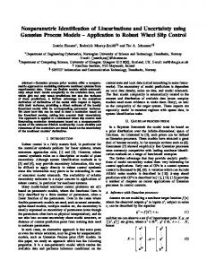
Fig. 1. Input/output noise model of the identification process. ( ) is the excitation signal, ( ) is the system response, x ( ) is the observation noise of the excitation signal, y ( ) is the output noise of the system to be identified, n ( ) and n ( ) are the measured (noisy) input and output signals and ( ) is the transfer function of the system.

x i

y i

yi

n i

n i

829

hi

Fig. 2. Model of the identification process. ( ) is the impulse response of the system, ( ) is the DFT of the excitation signal, n ( ) is the DFT of the measured (noisy) excitation signal, ( ) is the noise reduction filter, and est ( ) is the estimated impulse response.

h i

Xf

Rf

X f

Hf

Narduzzi and Offelli solve the deconvolution problem in the time domain [8]. A similar approach is reported by Bertocco et al. [9]. They define the optimization criterion based on the output reconstruction error. Consequently, the approaches assume perfect knowledge of the excitation signal. Dhaene et al. developed a method to optimize two parameters to obtain the best estimate for the transfer function of a system [10]. They separate the frequency region into pass, transition, and stop bands and define different noise factors. The optimum is defined by three conditions, which constrain the solution to a subspace; however, the choice of the concrete value remains subjective.

Fig. 3. Equivalent output noise model of the identification process. is the DFT of the noise sequence x ( ).

n i

N x (f )

Fig. 4. Simplified equivalent output noise model of the identification process. eq ( ) and eq ( ) are the equivalent noise and excitation signal sequences, and ( ) is the inverse filter.

n i

Kf

x i

III. OPTIMIZATION OF THE DECONVOLUTION FILTER Our aim is to develop a systematic algorithm to optimize the parameter(s) of the noise reduction filter. We assume both input and output observation noises. We developed the method for cases where the excitation signal is not perfectly known or it has to be measured. In previous works we developed a systematic optimization algorithm (model-based deconvolution), which is capable of optimizing more parameters [4]. However, the algorithm assumed an output noise, only. An extension of the model-based deconvolution algorithm is proposed in this paper to take both input and output observation noises into account in order to find the optimal level of the noise reduction. Our approach is based on approximation of the signal spectra [4], [13]. The spectral models are generated automatically by extracting the information from the measurement and, thus, no human interaction is required. The model of the measurement process is depicted in Fig. 1. A. Equivalent Output Noise Model The input/output noise model will be transformed to an equivalent output noise model. To do this, we will follow the flow of the estimation process rather than the signal flow. Thus, the input of the estimation process becomes the impulse response of the system (Fig. 2). By rearranging the noises they can be concentrated to the output of the system (Fig. 3).

Now we can define an equivalent output noise and an equivalent excitation signal (Fig. 4)

(1) is the Fourier transform of the equivalent where excitation signal, which is the measured (noisy) excitation is the equivalent output noise sequence, signal, and denotes convolution.

B. Measure of the Accuracy of the Solution The definition of the best solution is a subjective choice [12]. We will define it as the solution for which the squared summed error of the estimate of the impulse response is minimal. This error can be expressed both in the time and frequency domain, using the duality provided by the Parseval’s theorem:

(2)

830

IEEE TRANSACTIONS ON INSTRUMENTATION AND MEASUREMENT, VOL. 47, NO. 4, AUGUST 1998

where is the error energy, is the impulse response is the estimated impulse of the measurement system, is the sampling period, is the number of response, sampled points, and the capital letters correspond to the DFT’s of the signal sequences. is unknown, some Since the true impulse response approximations have to be done. Substituting the explicit form of the spectrum of the estimated impulse response into (2) we get

Fig. 5. Measured excitation signal and the output signal of the investigated digital oscilloscope.

its parameter(s) (3) is the transfer function of the measurement is the transfer function of the inverse filter, is the DFT of the measured excitation signal, is the DFT of the equivalent noise sequence, and is the phase angle of the two terms in the last sum. The error energy is thus split into three terms

where system,

(4) where the bias term is due to the distortion of the useful signal, term the noise term is due to the variance and the is due to the cross relation of the previous two terms. It has term can be neglected been shown in [13] that the under some mild conditions. The equivalent noise takes the form

(5) There is not much knowledge about the last term consisting of the phase information. The cosine term can be approximated or , or by its mean either by the upper or lower bound and value, which is zero if the noise sequences have zero mean value. We will assume zero mean value for the noise sequences, which is in most cases appropriate, and neglect the third term of (5). A further approximation is that instead of the absolute values of the signal and noise spectra, approximate spectral and . Thus, models will be substituted into we get the cost function, which will be minimized to set the by varying level of noise reduction of the inverse filter

(6) where subscript appx refer to an approximate model of the magnitudes of signal spectra. The noise spectra will be assumed white; thus, the magnitude will be modeled with a constant. The level of noise-model can be either a priori measured or extracted from the spectrum of the noisy signal. The transfer function will be modeled iteratively, starting from a rough model (straight frequency-domain division of the spectra of the output and the input measurements), and improving it in several steps by substituting the result of the estimated transfer function. More about this modeling procedure can be read in [4] and [13]. IV. EXPERIMENTAL RESULTS The impulse response of a high-speed sampling oscilloscope has been estimated. The oscilloscope operates in equivalent time sampling mode. The equivalent sampling frequency was 512 GHz. A step-like signal was applied to the input channel. The use of step-like signals has a partly historical, partly theoretical basis. Step-like signals excite the system in a broad frequency band and they are easy to generate. The repeatability of the signals is very good, which is a basic need because of the equivalent time sampling mode.

´ DABOCZI: NONPARAMETRIC IDENTIFICATION ASSUMING TWO NOISE SOURCES

Fig. 6. Magnitude of the DFT of the excitation signal and the model of the input noise.

831

Fig. 8. Initial approximation of the transfer function.

Fig. 9. Equivalent output noise model after 10 iterations. Fig. 7. Magnitude of the DFT of the system response and the model of the output noise.

The excitation was also measured with another high-speed oscilloscope, having a larger bandwidth. The price for the increased bandwidth is the loss of resolution. The measured excitation signal has thus a significantly higher noise level than the output signal of the investigated system. The measured input/output signals are depicted in Fig. 5. The step-like signals were extended with their mirrored version to make them time limited (Nahman–Guillaume technique [11]), since the signals are processed in the frequency domain. The DFT’s of the signals are shown in Figs. 6 and 7. Both the input and output noises are assumed to be white. Their levels were extracted from the measurement. The upper frequency band (from 75% of the Nyquist frequency to the Nyquist frequency) was assumed to contain only noise information. The average of the magnitude of the spectrum is considered as the level of the noise.

The magnitude of the transfer function is also required to compute the cost function. The initial approximation is the result of the frequency-domain division of the spectra of the Nahman–Guillaume extended output and input signals (Fig. 8). This model was improved in several iterations with the DFT of the new estimate of the impulse response. The model of the output noise and that of the equivalent output noise are shown in Fig. 9. The regularization method was used as the deconvolution filter with the second-order backward difference operator [11]. The inverse filter takes the form

(7) is the DFT of the second-order backward differwhere ence operator.

832

IEEE TRANSACTIONS ON INSTRUMENTATION AND MEASUREMENT, VOL. 47, NO. 4, AUGUST 1998

it assumes two observation noise sources (input/output noises). The method is based on approximate spectral models of the signals. The models are built algorithmically by extracting the information from the measurements. The measurement example was shown to support the theoretical results. The results can be used also for signal reconstruction tasks.

ACKNOWLEDGMENT The author would like to thank T. M. Souders, N. G. Paulter, and J. P. Deyst at the NIST for many fruitful discussions.

REFERENCES

Fig. 10.

Estimated transfer function of the system.

Fig. 11.

Estimated impulse response of the system.

The result of the deconvolution after ten iterations of improving the model of the transfer function is shown in Figs. 10 and 11. The high-frequency noise is not suppressed enough if only an output noise is assumed. Neglecting the input noise results in underestimating the necessary level of noise reduction. However, with the proposed cost function the solution is at the expected bias-noise tradeoff and the estimated bandwidth of the system complies with the expectation. V. SUMMARY The optimization of nonparametric identification was dealt with in this paper. The novelty of the proposed method is that

[1] A. N. Tikhonov and V. Y. Arsenin, Solution of Ill-Posed Problems. New York: Wiley, 1977. [2] T. K. Sarkar, D. D. Weiner, and V. K. Jain, “Some mathematical considerations in dealing with the inverse problem,” IEEE Trans. Antennas Propagat., vol. AP-29, pp. 373–379, Mar. 1981. [3] P. B. Crilly, “Error analysis with deconvolution algorithms,” IEEE Trans. Instrum. Meas., vol. 42, no. 1, p. 78, Feb. 1993. [4] T. Dab´oczi and I. Koll´ar, “Multiparameter optimization of inverse filtering algorithms,” IEEE Trans. Instrum. Meas., vol. 45, pp. 417–421, Apr. 1996. [5] N. S. Nahman, “Software correction of measured pulse data,” in Fast Electrical an Optical Measurements, J. E. Thompson and L. H. Luessen, Eds., NATO ASI Series. Boston, MA: Martin Nijhoff, 1986, pp. 351–417. [6] B. Parruck and S. M. Riad, “An optimization criterion for iterative deconvolution,” IEEE Trans. Instrum. Meas., vol. IM-32, pp. 137–140, Mar. 1983. , “Study and performance evaluation of two iterative frequency[7] domain deconvolution technique,” IEEE Trans. Instrum. Meas., vol. IM-33, pp. 281–287, Dec. 1984. [8] C. Narduzzi and C. Offelli, “A time-domain method for the accurate characterization of linear systems,” IEEE Trans. Instrum. Meas., vol. 40, pp. 415–419, Apr. 1991. [9] M. Bertocco, C. Narduzzi, C. Offelli, and D. Petri, “An improved method for iterative identification of bandlimited linear systems,” IEEE Trans. Instrum. Meas. Technol. Conf., Atlanta, GA, May 1991, CH29405/91, pp. 368–372. [10] T. Dhaene, L. Martens, and D. De Zutter, “Extended Bennia-Riad criterion for iterative frequency-domain deconvolution,” IEEE Trans. Instrum. Meas., vol. 42, pp. 176–180, Apr. 1994. [11] N. S. Nahman and M. E. Guillaume, “Deconvolution of time domain waveforms in the presence of noise,” Tech. Note 1047, Nat. Bureau Standards, Boulder, CO, 1981. [12] S. M. Riad, “The deconvolution problem: An overview,” Proc. IEEE, vol. 74, pp. 82–85, Jan. 1988. [13] T. Dab´oczi, “Deconvolution of transient signals,” Ph.D. dissertation, Tech. Univ. Budapest, Hungary, available as Tech. Rep. Tech., Ser. Electrical Engineering, Budapest, no. TUB-TR-94-EE12.

Tam´as Dab´oczi was born in Moh´acs, Hungary, in 1966. He received the M.S. and Ph.D. degrees in electrical engineering from the Technical University of Budapest, Hungary, in 1990 and 1994, respectively. He is currently a Senior Lecturer at the Department of Measurement and Instrument Engineering, Technical University of Budapest. His research area is digital signal processing, especially inverse filtering.