adaptive phased array radar signal processing using ...

RL-TR-97-223 Final Technical Report February 1998

^H,-^ %^^ ;

ADAPTIVE PHASED ARRAY RADAR SIGNAL PROCESSING USING PHOTOREFRACTIVE CRYSTALS University of Colorado Kelvin Wagner, Ted Weverka, Anthony Sarto, and Sam Weaver

APPROVED FOR PUBLIC RELEASE; DISTRIBUTION UNLIMITED.

19980415 091 AIR FORCE RESEARCH LABORATORY ROME RESEARCH SITE ROME, NEW YORK DUG QUALITY INSPECTED 8

This report has been reviewed by the Air Force Research Laboratory, Information Directorate, Public Affairs Office (IFOIPA) and is releasable to the National Technical Information Service (NTIS). At NTIS it will be releasable to the general public, including foreign nations. RL-TR-97-223 has been reviewed and is approved for publication.

APPROVED:

-"'c JAMES DAVIS Project Engineer

FOR THE DIRECTOR:

t

[ A'-Li. JL^DONALD W. HANSON, Director Surveillance & Photonics

If your address has changed or if you wish to be removed from the Air Force Research Laboratory mailing list, or if the addressee is no longer employed by your organization, please notify AFRL/SNDP, 25 Electronic Pky, Rome, NY 13441-4515. This will assist us in maintaining a current mailing list. Do not return copies of this report unless contractual obligations or notices on a specific document require that it be returned. ALTHOUGH THIS REPORT IS BEING PUBLISHED BY AFRL, THE RESEARCH WAS ACCOMPLISHED BY THE FORMER ROME LABORATORY AND, AS SUCH, APPROVAL SIGNATURES/TITLES REFLECT APPROPRIATE AUTHORITY FOR PUBLICATION AT THAT TIME.

Form Approved OMBNo. 07040188

REPORT DOCUMENTATION PAGE

needed, and completing and reviewing Public report™ burden for this collection of information is estimated to average 1 hour per response, including the time for reviewing instructions, searching existing data sources, gathering and maintaining the marters Services, Directorate for Information the collection of information. Send comments regarding this burden estimate or any other aspect of this collection of information, including suggestions for reducing this bu^en to Washmpton Hr. The individual weights compensate for the the phase shift between array elements produced by their physical separation, and adjust the response of the array to have a maximum at some particular angle. The interelement phase shift A between array elements for a narrowband signal arriving at angle 8, is given by A(f> =

27td . , , 2nd sin(0) = u

-. l.i

0

where Xrf is the RF signal wavelength, and d is the array element spacing. For phaseshift steering, each wn is simply a complex-valued multiplier, applying both an amplitude multiplication and a phase-shift of the form w„ = a„er"

2.4

For example, incrementally increasing the phase of each wn would apply a linearly increasing phase shift across the array, steering the angle of the antenna response. The TV adaptive weights provide iVDOFs. For the single plane wave incident RF signal at

Array Output

Figure 2.1. A phase-shift steered, linear phased-array antenna for narrowband array processing.

angle 0 shown in figure 2.1, the weight vector which maximizes the antenna response in the signal direction is the complex-conjugate of the signal vector X{u), (,.\

V*/\,\ d „-'Mu -ilkdu W = £W = [he ,e ...e -ikNdu]j

2.5

It is evident that for this case xnwn = 1 for all n. There is now an array gain of N resulting from the sum of the N antenna elements, and a cross-range resolution given by the effective size of the array, Icos(ö), where L is the length of the array and cos(0) is the steering angle. This linear array geometry provides the most straightforward example to further examine these properties of the formed beam. Initially assuming that the outputs of all N elements are uniformly weighted, in a receive scenario (essentially the same for transmit) the sum of all the element output voltages, Ear, for a single frequency sinwave input at frequency co will be8'9 Ear = sin(otf) + sin(cot + At + 2A0) + • • • + sin(ettf + (N- l)A)

= sm[tt» + (*->)A*/2]--L^L2

10

-2>n\d

-In/d

-n/d

0

n

ld 2n\d Wavevector kx

?>n\d

Figure 2.2. Array antenna pattern as a function of transverse wavevector component

where the interelement phase shift, A0, is given by equation 2.3. The first factor is just a phase shifted sinewave of frequency co, and the second is an aperture weighting function, which can be expressed in terms of the tranverse component of the incident wavevector, kx = ks'm(6), as _ sin[iVA0/2] _ sin[Mrfsin(g)/2] _ sm[Nkxd/2] W(kx) = sin[A^/2] sin[fc/sin(0)/2] sm[kxd/2]

2.7

which is plotted in figure 2.2. As shown in figure 2.2, W{kx) is periodic with a period of 2K/d. The heigth of the mainlobe is at W(0), and is equal to N, the number of elements in the array, which again demonstrates spatial processing gain. The first zero occurs when the argument of the numerator is equal to K, corresponding to kx = 2nN/d, and therefore the mainlobe width will be approximately 4K/Nd. This demonstrates that increasing the number of array elements reduces the mainlobe width and improves the spatial resolution of the array. The secondary maxima shown in figure 2.2 would in general produce erronious, or at best confusing signal returns. These maxima are referredto as "grating lobes"8'

9

and are produced whenever

ndsm(6)/X = 0,K,2K..., or correspondingly whenever kx = ±2n/d. For an incident 11

field of given wavelength Xrf, kx = 2^sin(A^)/Ar/-, and because |sin(A0)| < 1, k will have real values only between kx = ±2nj\f. This region is often referred to as "the visible region", or +90°. The primary means of grating lobe avoidance is to select closely spaced elements (d < A/2), so that none of the grating lobes lie in real space9' 10

. Irregular element spacing can also reduce grating lobes as well. Normalizing the square of equation 2.7 and setting the element spacing to

d = A/2, produces the antenna radiation pattern sin2[Afosin(6>)/2 tf2sin[*rsin(0)/2

2.8

Approximating the sine function in the denominator of equation 2.8 by its argument under the assumption that N is large, results in a radiation pattern of _,.. sin2riV^sin(Ö)/2l . 2,, , w N G(6) * -7-1 / )/'l = sinc (A^^sin(ö)/2) K [Nxsm(6)/2]2 '

.

2.9

Thus, for large N, the radiation pattern is essentially that of a uniform aperture, where the well-known sine2 far-field radiation pattern is related to the aperture via a Fourier transform relationship. In like fashion, the first sidelobe will be reduced from the power level of the main-lobe by approximately -13.5 dB. This result was based on the assumption that all of the elements were equally weighted before summation. Nonuniform weighting can be used to apodize the antenna and reduce sidelobe levels. For example the Dolphi-Chebyshev11, Taylor12, or cosine squared13 apodization functions are well known to reduce sidelobes, but possibly at the expense of main-lobe width increase. 2.1.2 True-time delay beam formation The inadequacy of phase-shift steering for broadband signal processing is exhibited by equation 2.3. The interelement phase shift A(j> is seen to be frequency

12

dependent; the higher the frequency, the higher the spatial phasor across the array which will be needed to control the beam. A different phase-shift is now required for each resolvable frequency over the signal bandwidth, however a single phase-shifter behind each antenna element provides only one. Thus each resolvable frequency is steered to a different angle, a condition known as "beam squint", which reduces the cross-range resolution of the array and increases sidelobe energy. An array can be considered broadband when the fractional bandwidth F = B/vlf of the array operating at center frequency vrf = c/X^ exceeds the center frequency wavelength divided by the antenna aperture L. In particular when B/vlf > XrfjL or when LB>c,

2.10

the beam rotates resolvably over the RF frequency bandwidth, and for large broadband arrays, when LB » c, beam squint is over many beamwidths. For broadband processing, time-delay elements are used to compensate for the actual time-of-flight difference of the signal between elements as the signal propagates across the array, which is the same for all frequencies. A simple example of true-time delay processing is shown in figure 2.3, where following each array element is a variable time-delay, and a real, multiplicative weight. The approach shown in figure 2.3 is not an architecture traditionally embraced by the RF community, but nevertheless multiple implementations of this architecture based on optical processing methods have been provided by various researchers. A straightforward approach to implementing the architecture shown in figure 2.3 is to route a modulated laser beam down various lengths of optical fibers14'

15 16

>

. Other

proposed methods include switching between free-space sections of variable lengths17'18, exploiting the frequency dependence of highly dispersive optical fibers19'20, and segmented mirror devices21. None of these approaches will be discussed in any detail here.

13

Variable Time-Delays

Real Weights

Output

Antenna Elements

Figure 2.3. Variable time-delay architecture for broadband array processing.

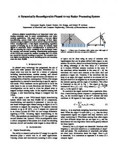
The traditional approach to true-time delay processing is done using discretely tapped delay lines, also known as a transversal filter1. This approach is shown implemented into a linear, 1-D antenna in figure 2.422>7. The true-time delay antenna in the figure can be viewed as a 1-D spatial array of transversal filters, each transversal filter providing the necessary temporal/frequency processing at each spatial sampling point along the aperture of the array. The function of the time-delays can be intuitively viewed as compensating for the time-of-flight variations across the array, which is most extreme for a signal arriving at endfire to the array. For the endfire case the array must be capable of processing signals over a time ta = L/c, corresponding to the time-offlight across the full array aperture, where L is the length of the array. The number of resolvable frequencies M, (equal to the number of required taps each with delay of T =

1/5) will then be M=BL/c = Bta

2.11

When multipath delays (with a maximum time delay tM) are also to be accounted for, Mmay need to be increased to BtM. 14

Figure 2.4. True-time delay implementation of phased-array antenna processes broadband signals. Depending upon the application, the number of taps can become quite large because the number of adaptive weights (and DOFs) is now equal toNxM. For the endfire case, an estimate ofN is obtained by considering that the array of length L will have an element spacing capable of Nyquist sampling the RF center frequency (Ar//2), leading to N = 2L/Xrf

2.12

As an example, consider a 1-D antenna system operating at a center frequency of 10 GHz, with a bandwidth of 2 GHz (F = 0.2). For an array aperture of L = 13.5 meters, it follows that TV = 1000, and M = 100. Thus this 1-D array would have a total of 100,000 weights, which is a formidable number to consider for real-time adaptive processing. 2.2 Adaptive Algorithms for Interference Cancellation The true processing power of the adaptive phased-array comes from the ability to adaptively suppress interference, while simultaneously optimally receiving the desired signal with the full antenna gain. The adaptive weights provide the DOFs

15

necessary to move the location of the antenna pattern nulls in the direction of unwanted interference. In general, an adaptive array with N degrees of freedom will be capable of nulling out N-l narrowband interfering sources, and still receive the desired signal. The primary performance metrics of the adaptive array are the signal-to-noise ratio (SNR) or the signal-to-interference-plus-noise ratio (SINR), and the convergence time. The SINR is often discussed in terms of the "improvement factor"23'24, or IF of the array, which is the ratio of the SINR of the adaptively formed output of the antenna to that of a single antenna element. In particular, the SINR and IF are defined as ~JNn

Desired Signal Power Interference Power + Noise Power

2.13

and IF =

SINR SINRe/emCT/

2.14

While there are a multitude of algorithms for controlling the weights of an adaptive array, there are fundamentally two distinct approaches which are taken. Direct algorithms, based on some criteria or measurement, with a single computation explicitly calculate the optimal weights as determined by a Wiener solution2 (i.e. those weights which maximize the SINR) and then implement these weights. Closed-loop algorithms are implemented recursively so that the system converges to the optimal weights for the given scenario. The former approach will be hereafter referred to as direct adaptive algorithms, and the latter as simply adaptive algorithms. The direct method is generally based on digitally computed signal statistics calculated over some finite temporal window and implemented open-loop, while the adaptive approach is generally errordriven and implemented closed-loop. As will be shown, the direct calculation of the optimal weights requires the calculation or estimation of correlation matrices as well as matrix inversions. If the number of weights NxM is small, a direct approach is sensible because the weights can be calculated and applied very efficiently in minimal time,

16

(although a finite temporal window is still necessary to estimate the correlation matrices). However, the matrix inversion operation is an order (NxMf process, and if this number is large, the direct approach can become computationally impractical and an adaptive algorithm which converges to the optimum weights is more sensible. This chapter will emphasize adaptive, error driven algorithms. An additional advantage to an adaptive approach is that because the weights are updated incrementally, the correlation matrices and inverses are not calculated explicitly, but are instead estimated from instantaneous values. By not calculating these matrices, there is an enormous advantage in terms of reduced computational memory requirements with the adaptive approach. The primary tradeoff with the adaptive approach is in terms of convergence time, which for certain signal environments may be very slow.

2.2.1 Adaptive Weight Calculation for Known Signal Environment When the properties of the signal environment are known, such as desired signal and noise spectra, and the AOAs of incident signals, the array output can be optimized by direct calculation of the optimum set of weights, Wopt. As will be shown in this section, a direct calculation of Wopt requires the calculation of two correlation matrices and a matrix inversion. Consider an N element, phase-steered array as shown in figure 2.1. The array output y{t) can be written as the sum of the weighted antenna element outputs25,

jw =J£rz e(t) = D(t) + U(t)-)(t) Output

Figure 2.9. Sidelobe canceller removes interference incident on primary antenna sidelobes.

essentially taking the difference between the desired and interference antenna patterns. This is shown conceptually in figure 2.10, where the auxiliary beam pattern is pointed towards the interference source corresponding to an incident direction of kin„ and has a scaled amplitude such that, when subtracted from the primary antenna pattern signal pointed at the desired signal in direction kd, the contribution of the inteference signal will be reduced in the output. Adaptively minimizing the difference between these two antenna patterns is analogous to redistributing the nulls of the antenna pattern in anglespace towards the directions of the interfering sources. It can be shown that the highest SNR is obtained when the total output power of the sidelobe canceller is minimized. As shown in figure 2.9, the auxiliary output y(i) is represented as the inner product of the input signal vector, X{t), and the weight vector W. The signals making up X(i) are assumed to be inteference sources only, where the interference is correlated between array elements (thermal noise is neglected here). This assumption of only interference power contained in the array elements is based on the

35

Primary Antenna Pattern

Difference Between Primary and Auxiliary Array Patterns

Auxiliary Antenna Pattern

/v^

ku Jammer

Reduced Sidelobe Antenna Response

hJ 1 Y\f\ f\r\

/N/^/TKl

ko Desired Signal

kv

kD

Figure 2.10. Conceptual represenation of sidelobe cancellation.

fact that usually the desired signal is much weaker than the interference, and that the omnidirectional acceptance pattern of the auxilliary array elements causes very little desired signal to be present in the received power from these elements. The signal output of the primary element is the sum of the desired signal D(t), and the interference source terms designated as U(t). The signals D{t) and U(t) are uncorrelated with each other, but U(t) is correlated with the interference sources of y{t) because they are from the same source. Note here that the processer output is the difference, or error, between the primary and auxiliary antenna components. This error is given by e{t) = D{t) + U(t)-y{t)

2.79

The weights are adjusted so as to minimize the expectation value of the squared error, and from equation 2.79, the expectation of the squared error is E[s\t)} = E[D\t)} + E[[U(t) - y(t)f] + 2E[D(t)[U(t) - y(t)]]

2.80

The cross-product term 2D{t)\U(t) - y(t)] goes to zero because D(t) is uncorrelated with both U(t) and y(t), resulting in E[£\t)] = E[D\t)] + E[[U(t)-y(t)f}

36

2.81

In order to minimize the residual error, it must be that the last term of equation 2.81 must be minimized, because D(t) is independent of W, and there would be no SNR advantage to minimizing D(t). Therefore, 2

^min] = F[D\t)} + E[(U(t)-y) min

2.82

Equation 2.82 yields the intuitive result that the error will be minimized when the auxiliary output y(t) is the best possible replica of the interference term U{t). The fact that the SNR is at a maximum when the total error is minimized is made evident by rewriting equation 2.79 as e{t)-D{t) = U{t)-y{t)

2.83

Thus, minimizing U(t)-y{t) is equivalent to minimizing the difference between the error and the desired signal, and therefore the minimum value of the error will be

4*^(0]=4^(0]

2 84

-

The result of equation 2.84 states that the minimum possible error is in fact the desired signal, and correspondingly the SNR will be a maximum when this occurs. It is important to point out that the implementation of the sidelobe canceller is based on two a priori pieces of information; the direction of the desired signal is known, and the strength of the desired signal is small compared to the integrated noise and interference power. The known signal direction allows the primary antenna to be pointed in the direction of the desired signal, and the weak signal assumption insures that the desired signal contribution from the auxiliary elements is minimal. If the desired signal is strong enough, with a significant contribution to the power received in the auxiliary elements, the sidelobe canceller will null this signal as well.

37

2.3 Optically Implemented Phased-Array Processing Algorithm The optically implemented phased-array processor developed in this thesis uses a modified version of the LMS algorithm to perform simultaneous beam formation and jammer cancellation. The intention of the algorithm is to provide a practical means of processing signals from very large phased-arrays, and is in part met by dramatically decreasing the number of required delay lines from N, where TV is the number of array elements, to only 2. Optical implementation of conventional (tapped) delay line structures for array processing as shown in figure 2.4 is often done with multichannel acousto-optic (AO) devices, one transducer per each antenna element, and therefore the number of AO channels required is equal to the number of antenna array elements. As a result, the limitations of multichannel AO technology32 typically limits the number of elements which can be processed to at most 32. In contrast, the delay line reduced, optically implemented LMS algorithm presented in this thesis, uses the inherent delay available in optical resonator cavities to achieve the required time delays necessary for wideband phased-array processing. This section demonstrates the equivalence between the adaptive weights of the optically implemented, modified LMS algorithm, and the weights used in the traditional tapped-delay line architecture presented in Section 2.2.4. It is important to point out how the modified algorithm closely resembles the WidrowHopf and Applebaum algorithms; the adaptive weights which are formed and the array output are equivalent, and the modified LMS algorithm produces the required number of DOFs to perform broadband, spatial-temporal processing for phased-arrays. However, there are important differences which are addressed at the end of this section. A schematic diagram of the modified LMS algorithm is shown in figure 2.11. The set of N tapped delay lines on the antenna elements that is used to produce the relative delayed output taps of the Widrow-Hopf algorithm of figure 2.7, have been replaced by a single tapped-delay line in the feedback, and distributed to all the elements in parallel. As in figure 2.7, the time integrated weights are calculated between the

38

incoming array signals and the relatively delayed feedback error signal. The weight wnm corresponds to the weight for the nth antenna element, at the mth delay, where now m corresponds to the relative delay of the feedback signal. The delay is implemented with a single AO device, and the weights are represented by the diffraction efficiencies of the time-integrated holographic gratings in the PRC. The products of the incoming unprocessed array signals and the weights at a particular delay are added, and these sums are Fourier transformed in space across delay value. Each output of the spatial Fourier transform is passed through a bandpass filter, and the outputs of the bandpass filters are summed to produce an output which is correlated with the reference signal r(t). The center frequency of the bandpass filters varies linearly across the filter array, and tuned so as to pass the signal which would have appeared at that position had instead the tapped delay line been used as the Fourier transform input. The Fourier transform operation is done simply in the optical domain with a lens, and the array of bandpass filters is obtained from a tilted or wedged Fabry-Perot resonator structure as discussed in more detail in Chapter 8. The adaptive network of figure 2.11 is shown being used as a jammer canceller. The delay, xe, that the reference signal passes through serves to decorrelate desired signals, which are assumed to be of broader bandwidth than the jamming sources. In this manner, while the broadband signals are present in the feedback signal, because they are delayed with respect to the incoming signals, they are decorrelated with the desired signals at the input of the array and do not build up appreciable weights. This suggests re should be chosen such that re »l/B, where B is the desired signal bandwidth. Using an AO cell for the feedback signal delay line results in the discrete weights of equation 2.66 becoming a continuous function of delay, where the delay is a proportional to the spatial variable

4Hl(xr w.

•

2,2

Ml

IT]

NO.

2.W

■s

0

MAT

Output

Figure 2.11. Schematic of optically implemented LMS algorithm.

velocity V of the AO cell. These continuous adaptive weights can be described by the time integral33

d2jdz2. For a weak dielectric perturbation this second derivative can be neglected (slowly-varying envelope approximation), resulting in to

p{z) ep^'e-x+^ + e2A2{z)ei,s>l eik°^x^

4 Q

The coupled-mode equations are obtained by using the orthogonality of the propagating modes. More specifically, multiplying equation 4.8 first by e1*^1(z)e'ü)'e"'ikBT e'g' rK^e. cq2cosQ B J

K„

k+wy

4.36

The sign of K will determine the direction of the two-beam coupling gain, and is dependent upon the orientation of the beams with respect to the crystal axis, the polarization of the beams, and the material electro-optic coefficients. Equations 4.34 and 4.35 can be solved for the intensities of the two signals by letting 4 = V^tf'*' and A2 = V^V*2 - This yields the steady-state coupled intensity equations48

.„(e1)i./1(x).-(fi^Öi]i^-ä/1(z) dz

\

cos(92)—I2(z) = +

kn0

J

10

s,7t sin(4>) | Ix (z)I2(z) -d/2(z) Xn o J

4.37

4.38

where is the spatial phase-shift between the dielectric perturbation and the incident intensity illumination pattern, typically 90 degrees. The intensity equations solved for the transmission grating geometry yield

I(z)-I (0 v«

^QHW) 4.39

l2[z)-i2[K)}e

rz cos

/](o)e-

/ ^+/2(0)

4.40

where the gain constant T is defined such that T = s,7T:sin((j>)/A,n0. The above equations indicate that for positive T, beam 2 undergoes coherent gain at the expense of beam 1, limited only by absorption. It is important to note that for