P7.2
1
ADAPTIVE ARRAY PROCESSING FOR MULTI-MISSION PHASED ARRAY RADAR
K. D. Le1 ,∗, R. D. Palmer2 , T. Y. Yu1 , G. Zhang2 , S. M. Torres1 ,3 , and B. L. Cheong2 1
School of Electrical and Computer Engineering, Norman, Oklahoma, USA School of Meteorology, University of Oklahoma, Norman, Oklahoma, USA 3 Cooperative Institute for Mesoscale Meteorological Studies, University of Oklahoma, Norman, Oklahoma, U.S.A. 2
Abstract As the use of phased array radars becomes more established for weather surveillance, adaptive array processing techniques will become more important to the weather radar community. Such techniques can be applied to phased array radars to improve angular resolution and also to suppress clutter compared to conventional beamforming methods. Thus, enhanced details of weather phenomena can be realized in terms of finer and better estimates of the reflectivity and radial velocity. This paper compares the performance of conventional beamforming to the performance of adaptive array processing based methods for a fully adaptive array and a partially adaptive array with six sidelobe-canceling elements, which is the configuration of the Multi-Mission Phased Array Radar (MPAR) of the National Weather Radar Testbed (NWRT) in Norman, Oklahoma. Different scenarios of fading clutter and clutter positions relative to the steering directions are considered. The simulated phased array concept uses a transmit beam that is wide in both angular directions to illuminate a large field of view and is thus termed an imaging radar. The receiver consists of individual antenna elements placed in a planar configuration. Time series signals for each antenna element are generated using a realistic radar simulator based on point-target scatterers, which flow and scatter according to a simulated environment produced from the Advanced Regional Prediction System (ARPS). Preliminary results show that, as expected, the performance of more sophisticated adaptive algorithms is superior compared to conventional beamforming, both in terms of angular resolution and clutter suppression.
1. INTRODUCTION The National Weather Radar Testbed, located in Norman, OK, has a 10-cm phased array radar that became operational in 2003 [Forsyth et al., 2007]. On∗ Corresponding author address: Khoi Duc Le, University of Oklahoma, School of Meteorology, 120 David L. Boren Blvd., Rm 4610, Norman, OK 73072-7307; e-mail:
[email protected], website: http://arrc.ou.edu
going research at the testbed using the radar includes beam-multiplexing [Yu et al., 2007], simultaneous aircraft tracking in weather [Yeary et al., 2007], crosswind measurement [Zhang and Doviak, 2007], and refractivity extraction from ground clutter scattering [Cheong et al., 2007a]. In particular, the availability of the radar has been beneficial for testing scanning strategies with faster update time that are more applicable in severe weather surveillance than the current scanning strategies of the WSR-88D. A proposed scanning solution consists of collecting fewer samples at one time for any position and to resample the position multiple times in one scan. Fewer samples are collected overall, yet since the samples are more decorrelated between resampling times, the required sensitivities of the estimated power and radial velocity are still maintained. A consequence of the strategy is that the number of contiguous timeseries samples is reduced, and the number of contiguous samples becomes problematic when it is less than the length of the impulse response of the ground clutter filter (GCF). As a result, clutter cannot be filtered effectively using the GCF, and the weather signal cannot be extracted. A practical solution to this dilemma of improving rapid update or clutter filtering is to use spatial filters, which can be implemented by using multiple-element receivers and weighting the respective signal of each element with a complex value to collectively produce destructive nulls, or near-zero gains, in the directions of the clutter sources. Since spatial filters require only the correlation value between the signals of the receiving element, they can be implemented without contiguous samples. If the receiver of a radar has multiple receiving elements and the time series of each receiving elements can be weighted, then the output signal of the phased array radar is given by
y
=
wH x
(1)
where x and w are the complex time series and weight vectors, respectively. In this paper, two spatial filters in the form of the sidelobe canceler (SLC) [Griffiths and Jim, 1982] and the minimum-variance distortionless response (MVDR), or Capon beamformer [Capon, 1969], are implemented and the results are compared to that
P7.2
2
from using a conventional 5th order elliptical temporal ground clutter filter (GCF). The weights of the SLC are obtained by solving
min ||ym −
H wSLC xSLC ||2 ,
(2)
where ym is the time series of the main channel, which is obtained by conventional Fourier beamforming on an array of receivers, and wSLC and xSLC are the complex time series and weights of the sidelobe canceling elements. The weights of the Capon beamformer is obtained by solving
min ||y||2 subject to wH e = 1,
(3)
where e is the steering vector. In general, the number of SLC elements are much less than that of the Capon beamformer and is correspondingly less computationally intensive. The weather scenario considered is a tornadic supercell dominated by ground clutter. The effect of scanning elevation angle, clutter fading, and position of SLC elements are considered. The number of sidelobe canceling elements is six while the number of elements in the Capon beamformer is 1088. Currently, time series data cannot be readily obtained from the SLC elements on the MPAR, so validation of the discussed spatial filters is achieved using the available Turbulent Eddy Profiler (TEP) [Mead et al., 1989; Palmer et al., 2005], which is a vertically pointing radar. The results from processing the TEP data and show the potential of the method.
2.1. Simulator The three-dimensional model of Cheong et al. [2007b] is used to generate the time series for the antenna elements. The model uses atmospheric values of reflectivity and flow derived from ARPS to simulate a realistic scattering field. The volume of the field is defined by the scanning region and is padded with a width of half a beamwidth on each side of the angular scanning direction and half a range gate length in the range direction. Fifty thousands point targets are initially randomly placed within the simulated volume, and the position of each scattering target is updated for each sampled pulse using motions derived from the ARPS flow field. In the model, the time series are produced by the radar first transmitting a short burst of energy to radiate the scatterers. The radar is immediately switched to a listening mode to collect the returned echo. The signal at the receiving element V (τs , mTs ) is a sum of all the scattered signals, namely
V (τs , mTs )
=
PN −1 k=0
Ak exp[−jψ k ] + n(τs , mTs )
(4) where A is proportional to the position, range weighting function, beam weighting function, and expected reflectivity. The phase of the k th scatterer is ψ k and depends on the two-way path length, accumulated propagation phase, scattering phase, and transmitted and demodulated phase. N is the number of scatterers, and n(τ, mTs ) is the receiver noise. The signal is periodically measured for the train of transmitted pulses.
2. SIMULATION STUDY 2.2. Results A tornadic scenario as generated by the ARPS numerical weather prediction model initiated using the 197705-20 Del City sounding is imaged using a phase array with the specifications listed in Table 1. The radar samples the scene at 0.5◦ angular azimuthal spacing, for 15 range gates, and for the 0.5◦ , 1.5◦ , 2.5◦ , and 3.5◦ elevation angles. The storm is approximately 32 km from the radar, while the radar is pointed 10◦ above the ground to emulate the MPAR configuration. The simulated array has less than 1,100 elements compared to the Aegis SPY-1A antenna that has more than 4,000 elements. The selected number of simulated elements was reduced for simulation complexity issues. The tornado is located at (33,1) km based on the observed position with the lowest surface pressure. Additionally, the above ground level (AGL) for the 0.5◦ , 1.5◦ , 2.5◦ and 3.5◦ elevation scanning angle and the 32 km range is approximately at 280 m, 840 m, 1.4 km, and 2.0 km, respectively. Moreover, the angular width of a 1◦ beamwidth at this range is approximately 560 m across.
The imaged fields using SLC and Capon beamforming are compared to the imaged fields of Fourier w/o Clutter, Fourier w/ Clutter, and the imaged field obtained by processing the time series signal obtained from Fourier w/ Clutter using the described GCF. The ability of the SLC and Capon beamformer to suppress clutter is examined for variations in elevation angle, amount of clutter fading, and positions of SLC element. A benefit of using the GCF is that the performance for extracting the weather signal is based on the assumptions that the clutter return has zero or near-zero radial velocity signature while the weather signal has non-zero radial velocity signature, the clutter filter width contains the clutter signal, and the stopband suppression is sufficient. When these assumptions are satisfied, ground clutter is rejected and the weather signature is extracted with precision. However, when these conditions are not met, the filtered signal can be worse than that obtained using spatial filters. On the other hand, the performance of the spa-
P7.2
3
Table 1: Phased array simulation parameters simulated volume (Zonal x Meridional x AGL) number of atmospheric scatterers number of ground clutter scatterers equivalent reflectivity of clutter scatterer transmit antenna receive aperture (width x height) number of received elements pulse repetition frequency aliasing velocity number of pulses range resolution
tial filters, in particular the SLC and Capon beamformer, depends on variables such as number of elements, element spacing, number of adaptable elements, array aperture, noise level, number of time samples, as well as spatial and temporal variation in the scattering field.
2.2.1) Effects of Elevation Angle In the discussion of this subsection, the amount of clutter fading is fixed at 0.1 ms−1 . Preliminary results are provided in Figure 1. For this fading value, residual clutter is observed for different elevations only when the received power is extremely strong. This situation correlates well to conditions where the imaged position of Fourier w/ Clutter has power values greater than 55 dB and the lower scanning elevation angles of 0.5◦ , 1.5◦ , and 2.5◦ . Since the sidelobe level increases to the mainlobe, the contribution of clutter in the return signal is expected to be higher for the lower elevation angles. At the lowest elevation, residual clutter exists and is comparable in magnitude to the weather signal. Based on the results and as expected, the performance of the GCF is independent of the steered direction. On the other hand, the six-element SLC is particularly sensitive to the relative position of clutter and steered beam direction. As the mainlobe is steered closer to the surface, the angular separation to the mainlobe becomes narrower. The ability of the SLC to affect the beampattern becomes prohibitively difficult as is evident when the beam is closer to the ground. The clutter is the dominant imaged feature at the lowest elevation angle. On the other hand, the Capon beamformer, which has a much larger number of elements and weight combination can alter its beampattern to suppress clutter while extracting the weather feature even to the lowest eleva-
7 (km) x 7 (km) x 5 (km) 50,000 1,000 80 dBZ wide-beam 3.6 m x 3.8 m 1094 1000 (Hz) 23.4 ms−1 250 235 m
tion angle. This is observed even in the updraft region of the storm.
2.2.2) Effects of Fading Clutter
Ground clutter sources, as they move or are moved by the surface wind, introduce close to zero but non-zero radial velocity signatures. The motion causes fading, or decorrelation, of the return signal in time, impacts the spread of the clutter signal, and changes the required width of the GCF. While the amount of fading then determines the width of the clutter filter, the amount of clutter that is filtered is determined by the width and attenuation values that are set during the design of the GCF. Additionally, the amount of fading changes the decorrelation time of the received signal and affects the correlation values used in calculating the spatial filter weights. The effects of filtering using a GCF with fixed width and stopband attenuation, and with the spatial filters, are plotted in Figure 2. As is expected, the amount of residual clutter increases with the amount of clutter fading and it is evident as an increase in power and a bias of the radial velocity towards zero. A similar effect occurs with the SLC as clutter fading increases. On the other hand, while the imaged reflectivity field obtained using Capon beamforming changes, the imaged radial velocity field contains values that are further away from zero. The effect on the radial velocity of Capon beamforming is contrary to those obtained using GCF and SLC. An explanation is that the estimate of the spatial correlation used in the Capon beamformer improves with the increased amount of fading.
P7.2
4
°
°
1 0 −1 −2
Fourier w/ Clutter
2 1 0 −1 −2
2
GCF
1 0 −1 −2
2
SLC
SLC
1 0 −1
2 1
Capon
Capon
Meridional Distance (km)
−2
0 −1 −2
30 31 32 33 Zonal Distance (km)
20
25
30 31 32 33 Zonal Distance (km)
30
35
30 31 32 33 Zonal Distance (km)
40
45
50
30 31 32 33 Zonal Distance (km)
55
60
Power (dB)
Meridional Distance (km)
2
Meridional Distance (km)
Fourier w/o Clutter
θ=3.5
Meridional Distance (km)
Fourier w/o Clutter
Meridional Distance (km) Meridional Distance (km)
Fourier w/ Clutter GCF
Meridional Distance (km)
°
θ=2.5
Meridional Distance (km)
°
θ=1.5
Meridional Distance (km)
°
θ=0.5
°
°
°
θ=0.5
θ=1.5
θ=2.5
θ=3.5
30 31 32 33 Zonal Distance (km)
30 31 32 33 Zonal Distance (km)
30 31 32 33 Zonal Distance (km)
30 31 32 33 Zonal Distance (km)
2 1 0 −1 −2
2 1 0 −1 −2
2 1 0 −1 −2
2 1 0 −1 −2
2 1 0 −1 −2
−20
−15
−10
−5
0
5
Radial Velocity (ms−1)
10
15
20
Figure 1: Power and radial velocity as imaged for the elevation angles of 0.5◦ , 1.5◦ , 2.5◦ , and 3.5◦ . The left panel consists of estimated power plots, and the right panel consists of radial velocity plots. Regions containing storm structure are associated with continuous power and radial velocity values, whereas regions of clutter are associated with speckled power and zero radial velocity values.
2.2.3) Effects of SLC positions
The effective receive beampattern is a function of the complex weight, position, and angular response of each receiving element. For the SLC and the phased array under consideration, the weights of 1088 elements that make up the main channel are fixed and only the weights of six sidelobe elements are variable. As a result, the shape and response of the mainlobe should not significantly change unless the summed complex weights of the SLC elements become relatively significant compared to the summed weights of the main channel. For the minimization technique considered for the SLC, this condition did not exist and only the sidelobe levels are significantly changed.
The effects of ground clutter suppression due to SLC positions are considered for four SLC configurations: MPAR, Horiz, Diag, and Vert. The positions of the elements of each configuration are plotted in Figure 3. The amount of clutter fading is 0.1 ms−1 . The results are compared to the fields of Fourier w/o Clutter and those obtained using the GCF, and they are plotted in Figure 4. The amount of clutter is reduced the most for the Diag configuration and the least for the Vert and Horiz configuration. Though the beampattern is not plotted, it is believed that the sidelobe level obtained along the ground is lowest using the Diag configuration.
P7.2
5
−1
−1
Fourier w/ Clutter
−2
2 1 0 −1 −2
2
GCF
1 0 −1 −2
2
SLC
1 0 −1 −2
2
Capon
1 0 −1 −2
20
25
30 31 32 33 Zonal Distance (km)
30
35
40
45
55
60
σ=0.1 (ms )
−1
σ=1.0 (ms )
2 1 0 −1 −2
2 1 0 −1 −2
2 1 0 −1 −2
2 1 0 −1 −2
2 1 0 −1 −2
30 31 32 33 Zonal Distance (km)
30 31 32 33 Zonal Distance (km)
50
Meridional Distance (km)
Fourier w/o Clutter
0
Meridional Distance (km)
1
Meridional Distance (km)
2
30 31 32 33 Zonal Distance (km)
−1
σ=0.0 (ms )
σ=1.0 (ms−1)
Meridional Distance (km)
σ=0.1 (ms−1)
Meridional Distance (km)
Meridional Distance (km) Meridional Distance (km)
Fourier w/ Clutter GCF
Meridional Distance (km) Meridional Distance (km)
SLC Capon
Meridional Distance (km)
Fourier w/o Clutter
σ=0.0 (ms−1)
−20
Power (dB)
−15
30 31 32 33 Zonal Distance (km)
−10
−5
0
5
30 31 32 33 Zonal Distance (km)
10
Radial Velocity (ms−1)
15
20
Figure 2: Power and radial velocity as imaged for the clutter fading of 0.0, 0.1, and 1.0 ms−1 . As the amount of fading increases, the temporal decorrelation of the signal is shorter and imaged power and radial velocity fields are smoothed.
MPAR
Horiz
Diag
Vert
2 z (m)
1 0 −1 −2 −2 −1
0 1 x (m)
2
−2 −1
0 1 x (m)
2
−2 −1
0 1 x (m)
2
−2 −1
0 1 x (m)
2
Figure 3: Element positions for four SLC configurations. The mainlobe elements are marked ’x’ and the SLC elements are marked ’*’.
3. VALIDATION USING TURBULENT EDDY PROFILER The Turbulent Eddy Profiler used for validating the simulation is a 915-MHz radar that consists of a transmit horn
antenna and up to 64 receive microstrip patch antennas. The elements are separated by approximately 0.57 m. The pulse repetition frequency is 35 kHz and 250 co-
P7.2
6
Power Radial Velocity
GCF
SLC−MPAR
SLC−Horiz
30 31 32 33 Zonal Distance (km)
30 31 32 33 Zonal Distance (km)
SLC−Diag
SLC−Vert
Capon
2 1 0 −1 −2
Meridional Distance (km)
Meridional Distance (km)
Fourier w/o Clutter Fourier w/ Clutter
30 31 32 33 Zonal Distance (km)
20
30 31 32 33 Zonal Distance (km)
25
30
35
30 31 32 33 Zonal Distance (km)
40
45
50
55
Power (dB)
60
−20
−15
30 31 32 33 Zonal Distance (km)
−10
−5
0
30 31 32 33 Zonal Distance (km)
5
10
15
30 31 32 33 Zonal Distance (km)
20
−1
Radial Velocity (ms )
Figure 4: Power and radial velocity as imaged for different four configurations of SLC element positions. The positions of the SLC elements are important factors that determine the effective sidelobe level in the direction of the clutter sources.
herent samples were integrated to produce an effective sampling time of 7.14 ms to produce an aliasing velocity of 11.48 ms−1 . The range resolution of this radar is approximately 33 m. Fifty-eight gates were collected for a total range imaged distance of approximately 1750 m. The discussed clutter processing techniques were applied to a series of data collected on 2003-06-15 from 17:13 UTC to 17:34 UTC. During this day, the time series were available for 56 total elements. In the analysis, the center 50 elements were used along with Fourier beamforming to obtain the main channel signal, and six elements placed in the MPAR configuration was used as sidelobe canceling elements. A 5th order GCF with 1 dB passband ripple, 1 ms−1 passband edge, and 70 dB stopband attenuation was used. The results are plotted in Figure 5. The imaged fields using Fourier beamforming contain ground clutter up to approximately 400 m AGL. The large features that are present from the surface to about the top of the imaged field are convective plumes, which are caused by surface heating and mixing with the stable free atmosphere above. Aerial clutter are present and are characterized by stronger than 20 dB power and non-zero radial velocity values. Vertical lines are products of random surges in the power level of some of the receivers probably caused by interference. The fields obtained by filtering with the GCF contain a much lower level of clutter. The horizontal layer of clutter above 1100 m is gone. The ground clutter at the surface is attenuated to a height of approximately 60 m. The radial velocity field is more pronounced and tend to be more biased away from zero. Both weather and clutter
signals are removed when both have radial velocity signatures within the width of the GCF as are marked by the temporal discontinuity of the convective plume that consists of sudden decreases in power and random radial velocity values. Some examples of regions with power voids are located between 1000 m and 1700 m at times 17:14, 17:16, 17:17, and 17:21 UTC. The imaged fields of SLC are different than that of the fields obtained using GCF. The height to which ground clutter is attenuated is lower, and it is near the ground. The clutter layer above 1100 m is still present but it is attenuated. Some of the aerial clutter are filtered, while the region of power for others are decreased. The convective plumes are temporally more continuous compared to that obtained using GCF. The imaged radial velocities have lower overall radial velocity values, which are more consistent with the mostly turbulent flow of the convective plumes. Compared to the fields obtained with Capon beamforming, the reflectivity values are larger and they are expected. The ground clutter as well as the clutter layer above 1100 m is attenuated at a more pronounced level. The aerial clutter has almost completely been attenuated. The structure of the radial velocity fields obtained using the two methods, on the other hand, are very similar to each other.
4. CONCLUSIONS The SLC and Capon beamforming techniques have been applied in both simulation with the NWT MPAR configuration as well as validation using the TEP radar. While the results obtained using Capon beamforming
P7.2
7
Figure 5: Power and radial velocity as imaged with the TEP. The data are collected on 2003-06-15 from 17:13 UTC to 17:34 UTC.
are the most realistic in terms of producing the best weather features in simulations, the results obtained using the six SLC elements provide evidence that ground clutter can be suppressed and as well as the GCF in some cases. The results obtained by processing the time series data of the TEP radar are more promising. The power and radial fields obtained using SLC are heuristically more similar to that obtained using Capon beamforming than that using GCF.
5. ACKNOWLEDGMENT
This work was supported by the National Severe Storms Laboratory through cooperative agreement NA17RJ1227.
References Capon, J., 1969: High-Resolution FrequencyWavenumber Spectrum Analysis. Proc. IEEE, 57(8), 1408–1418. Cheong, B., R. Palmer, C. Curtis, T.-Y. Yu, D. Zrnic, and D. Forsyth, 2007a: Refractivity Measurements From Ground Clutter Using the Nation Weather Radar Testbed Phased Array Radar. San Antonio, TX. Cheong, B., R. Palmer, and M. Xue, 2007b: A TimeSeries Weather Radar Simulator Based on HighResolution Atmospheric Models. J. Atmos. Oceanic Technol., submitted. Forsyth, D., J. Kimpel, D. Zrnic, S. Sandgathe, R. Ferek, J. Heimmer, T. McNellis, J. Crain, J. Belville, and W. Benner, 2007: Update on The National Weather Radar Testbed (Phased-Array). San Antonio, TX.
P7.2
Griffiths, L., and C. Jim, 1982: An Alternative Approach to Linearly Constrained Adaptive Beamforming. IEEE Trans. Anten. Prop., AP-30(1), 27–34. Mead, J., G. Hopcraft, S. Frasier, B. Pollard, C. Cherry, D. Schaubert, and R. McIntosh, 1989: A VolumeImaging Radar Wind Profiler for Atmospheric Boundary Layer Turbulence Studies. J. Atmos. Oceanic Technol., 15(4), 849–859. Palmer, R., B. Cheong, M. Hoffman, S. Frasier, and F. Lopez-Dekker, 2005: Observations of the SmallScale Variability of Precipitation Using an Imaging Radar. J. Atmos. Oceanic Technol., 22(8), 1122– 1137. Yeary, M., B. McGuire, Y. Zhai, D. Forsyth, W. Benner, and G. Torok, 2007: Target Tracking at The National Weather Radar Testbed: A Progress Report on Detecting and Tracking Aircraft. San Antonio, TX. Yu, T.-Y., M. Orescanin, C. Curtis, D. Zrnic, and D. Forsyth, 2007: Beam Multiplexing Using the Phased-Array Weather Radar. J. Atmos. Oceanic Technol., 24(4), 616–626. Zhang, G., and R. Doviak, 2007: A Theory for the Phased-Array Weather-Radar to Measure Crossbeam Wind, Shear and Turbulence. San Antonio, TX.
8


![[PDF] Download Phased-Array Radar Design: Application of Radar ...](https://m.moam.info/img/260x300/pdf-download-phased-array-radar-design-application_6477d7f2097c4786708c28fc.jpg)