Application Framework for Computational Chemistry (AFCC) applied to New Drug Discovery J. Tindle, M. Gray*, R.L. Warrender, K. Ginty, P.K.D. Dawson* Department of Computing, Engineering and Technology Department of Pharmacy, Health and Well-being * Faculty of Applied Sciences, University of Sunderland, St. Peter’s Campus, Sunderland, SR6 0DD, U.K. (e-mail:
[email protected]) ABSTRACT
This paper describes the performance of a compute cluster applied to solve three dimensional (3D) molecular modelling problems. The primary goal of this work is to identify new potential drugs. The paper focuses upon the following issues: computational chemistry, computational efficiency, task scheduling and the analysis of system performance. The philosophy of design for an application framework for computational chemistry (AFCC) is described. Various experiments have been carried out to optimise the performance of a cluster computer, the results analysed and the statistics produced are discussed in the paper. Keywords: High performance computing HPC, new drug discovery, molecular modelling, computational chemistry, parallel computing, compute cluster
1. INTRODUCTION Computational methods have been developed that allow researchers to carry out comprehensive investigation of molecules and their reactions. Molecular modelling allows the researcher to observe biological reactions and the associated dynamics providing highly accurate descriptions of the relevant interatomic forces. In most cases it is computationally expensive to solve the high level quantum chemistry models. Chemists are now able to investigate the properties of chemical structures at the molecular level. The aim of the research described in this paper is to discover new drugs that targets particular cells and cures diseases at the cellular or genetic level. This paper describes the performance of a compute cluster applied to solve a large number of molecular models. The paper considers factors such as the computational chemistry and molecular modelling, computational efficiency, task scheduling and the analysis of cluster system performance. The design of an application framework for computational chemistry (AFCC) research is discussed.
The University of Sunderland have recently installed and commissioned a general purpose high performance compute cluster in the Computing department. This development is based upon Microsoft High Performance Computing HPC Servers and the Compute Cluster Pack [1][2]. The design of the cluster computer was completed by University of Sunderland (UoS) and Dell engineers [3][4], refer to Appendix 1. A more detailed description of the cluster system hardware and software configuration may be found in the paper by Ginty [3]. The UoS cluster computer has recently been used to complete some 3D computer graphics (CG) modelling projects [5]. Staff employed within the departments of Computing and Pharmacy collaborated upon this research.
2. MOLECULAR MODELLING Molecular modelling software allows the user to select atoms from the periodic table and to place them in a three dimensional workspace. In most modelling systems it is possible to build a three dimensional molecular structure by using a colour graphics user interface (GUI), refer to Figure1. The initial position of the atoms is normally determined by the user calling upon common sense and experience. In all cases the actual position that the atoms assume in the real world is determined by the Laws of Physics. Computational chemistry is a general name for computer based algorithms that may be used to solve this type of problem. There are numerous algorithms that may be deployed and normally this involves computing the minimum value of an energy function to find the optimum solution.
Figure1 Molecular Modelling Workspace For complex structures in many cases the rate of convergence is relatively slow and it is therefore often necessary to employ high performance computing methods to produce solutions in a reasonable period of time.
2.1 Model Convergence Time There are three principle factors that influence the time required to produce an acceptable solution.
The initial position of the atoms selected by the user. This initial set of atomic positions is the seed for the numerical solver algorithm embedded in Gaussian_09. The number of heavy atoms in the model of the molecular structure. The basis set and the method deployed, for example, the molecular mechanics protocol which is intrinsically fast or the ab initio method MP4 that is relatively slow [13,14].
A system that accurately models the Schrodinger Equation will normally require a long time to produce a good solution whereas more approximate methods produce solutions more rapidly. T is proportional to K * An Where T is the time to produce a solution K is a constant that is associated with method in use A is the number of heavy (non-hydrogen) atoms n is a scalar value of 4 When large numbers of atoms are involved in a model the time taken to generate a solution can be very long.
3. NEW DRUG DISCOVERY By using HPC methods and computational chemistry it is possible for the user to create a set of new potential drugs. The output data produced by the solver algorithms allows the user to evaluate each potential candidate and select the best for production and further testing. In this scenario it is only necessary to manufacture and test the best candidate molecular structures and the data associated with poor models may be discarded or archived. By evaluating a large number of the most promising models and selecting only the most promising cases it is possible to minimise production and testing costs. The cost of developing a new drug can run into hundreds of millions or even several billion dollars. The traditional process will usually take 10 or more years and result in the synthesis, purification and biological evaluation of ten thousand or more new compounds in order to produce a single viable clinical candidate. In order to reduce the costs implicit within the above, the pharmaceutical industry has invested heavily in computational approaches to drug discovery. These approaches often rationalise existing biological data to make informed choices as to the next series of compounds to make, so called Pharmacophore or Quantitative Structure Activity Relationship (QSAR) approaches. Alternatively, where good quality structural information is available regarding the intended biological target molecule, usually a particular enzyme, receptor protein or strand of DNA/RNA, a research team can embark upon a programme of so called Rational Drug Design. Rational Drug Design comes in several subtypes, the details of which are beyond the scope of this paper. However, they all operate by defining a region of space within the target biomolecule within which the drug candidate must fit. The usual analogy for this is that we are
trying to find a specific key (the drug candidate) that fits a particular lock (the drug target). Thus the drug candidate must be the correct size and shape to snugly fit within the available space in order to maximise the potential for interactions between drug and target without being too big to fit at all. Along with the relatively crude considerations that must be made with regards to a complementary shape between lock and key we must also consider the complementarity or otherwise between the surface electrostatic potentials of the two molecules. All molecules whether natural or synthetic are made from atoms and these atoms are made in turn from three components: protons, neutrons and electrons. The protons which are positively charged and neutrons which are electrically neutral form a dense nucleus within the heart of each atom which is surrounded by a swarm of negatively charged electrons. However, when we put atoms together to make molecules certain atoms attract more of the electron density towards themselves on average than others. This leads to the surface of typical molecules being electron rich and electrostatically negative in some areas and electron deficient or electrostatically positive in others. If we were to find molecules with the correct shape to fit to our binding site but would place regions of high electron density in contact with one another, Coulomb’s Law dictates that the two molecules would repel and thus binding would not be able to take place. Similarly, repulsion would take place between molecules with a significant degree of electrostatically positive contact. Productive binding can thus only take place when the drug and drug target display regions of opposite charge on the electrostatic surfaces that would be in contact with one another when the drug docks into the target binding site. Many programmes have been developed that are able to assign surface electrostatic potentials of molecules based upon a qualitative knowledge of the properties of their constituent atoms and then attempt to dock them together, and many new compounds in the clinic have been designed with the aid of these techniques. However, the ability of the computer to assign these charges and other properties of the molecules in question is entirely dictated by parameter sets stored within the computer. In reality, it is known that when two molecules come into contact with one another they perturb the electron distribution within one another. This interplay between the electrostatic potentials of the two molecules in many instances is rather subtle but in some cases can lead to unexpected effects when the two molecules are allowed to bind to one another in real life. Moreover, many drugs that have long been on the market, such as aspirin and penicillin, operate by causing a chemical reaction between themselves and their target molecules alongside the initial binding event. These effects are much more difficult to anticipate and are often impossible to predict using the standard software in the industry based upon the traditional parameterised molecular mechanics (MM) approaches. Problems such as reactivity and mutual polarisability that occur when two molecules come into intimate contact are however able to be tackled using Quantum Mechanics (QM). Quantum mechanical programmes such as Gaussian operate by finding approximate solutions to the Schrodinger Equation for collections of atoms and molecules using only physical constants such as the masses of subatomic particles and the speed of light. This means that there are no limitations or biases in these calculations from pre-determined parameter sets and the true nature of the interactions and reactions between molecules becomes realisable.
However QM methods are highly computationally resource intensive to the extent that while programmes for carrying out such calculations have been available for many years their implementation in biologically relevant problems such as drug design has not been feasible until recently due to the size and complexity of these molecules. Even now full QM approaches are not deemed to be cost effective for medium or large biological molecules and thus hybrid, or so called QM/MM approaches, have been developed. In a typical QM/MM calculation the drug or natural ligand to be studied is treated quantum mechanically, as are the parts of the target molecule which make up the binding site. The rest of the target molecule is treated using more traditional MM methods. 3.1 Parallel Processing To identify a new potential drug a large number of jobs must be evaluated. This results in many hundreds of or even thousands of jobs being presented to the compute cluster for processing. Each job takes a finite time from perhaps a few hours up to many days 3.1.1 Compute Cluster Multiprocessing CCM. If all the resources of the compute cluster are focused upon single job individual solutions are usually produced very rapidly. This method is termed compute cluster multiprocessing CCM. However, the operation of splitting the task between nodes results in an increased communication overhead and normally a reduced level of efficiency. 3.1.2 Symmetric multiprocessing SMP An alternative approach is to suffer the longer time delay incurred and allocate a single job to each Compute Node for processing. The authors selected symmetric multiprocessing SMP for this work. The SMP approach works in conjunction with a job scheduler so that many jobs can run in parallel. The use of the scheduler ensures that there is no delay between the allocation of new jobs to Compute Nodes. SMP techniques that optimise the use of CPU cores and available RAM have been employed to ensure that CPU usage of 100% is normally achieved at each Compute Node.
4. COMPUTATIONAL CHEMISTRY AND GAUSSIAN Professor John Pople designed the first version of the Gaussian computer program to make his computational techniques easily accessible to researchers. The use of Gaussian makes possible the theoretical study of molecules, their properties, and how they act together in chemical reactions. The Gaussian program has been continuously developed by many researchers and today it is a software product that is used by thousands of chemists. Professor John Pople was awarded the Nobel Prize in chemistry in 1998 for his pioneering contributions in developing computational methods. Researchers can use Gaussian_09 to investigate the following topics [8].
Comprehensive investigation of molecules and their reactions Predicting and interpreting spectra Predicting optical spectra including hyperfine spectra Investigate thermo chemistry and excited state processes
Gaussian_09 allows solvent effects to be taken into account when optimising structures and predicting most molecular properties Modelling NMR
In the past chemists used standard laboratory methods to undertake research, for example by using chemical compounds, solvents, test tubes and heat sources. It is now possible to complete much of this practical research work by using powerful computers and computational chemistry software. The application of computation chemistry has many advantages mainly by helping to reduce the need for access to expensive laboratory time, test equipment and chemicals. From experience the authors have found that it takes about five minutes to manually prepare a single Gaussian_09 job to be sent to the scheduler prior to execution on the cluster computer. The manually preparation of jobs for execution is a standard approach often adopted by many research groups. This approach is most appropriate where a relatively small number of jobs are being processed by the scheduler, for example less than one hundred jobs. The authors of this paper are working with a group of six research chemists working upon drug development. These researchers have produced large number of jobs in batches of various sizes for execution on the cluster computer. A single batch contains typically between one hundred and five hundred Gaussian_09 jobs. It is anticipated that the total number of jobs that will eventually be processed on the cluster will be of the order ten thousand for any given development. To date more than six thousand jobs have been completed. In this paper the initial two hundred and seventy six jobs have been analysed to determine the performance characteristics of the cluster computer. The development of the AFCC allows a large batch of jobs to be easily submitted to the cluster normally within a few minutes thereby saving valuable time. By using the computational chemistry techniques researchers are able to carry out a series of experiments on a particular molecular structure (compound or solvent) in a manner similar to that employed in a conventional laboratory facility. AFCC employs a scheme where ‘the human is in the loop’. In a typical scenario the researcher inspects the output results obtained for chemical structure of interest and determines the direction of future experimentation. A range of factors are taken into account. The most important factor is usually the molecular structure which can be inspected and manipulated in three dimensions by using GaussView GUI. By inspecting the results it is also possible to inspect the bonds between atoms, electron transition states, spectra and photo luminescence effects when a compound is mixed in a solution. In AFCC there is no limit to the number of experimental steps that may be deployed. To date the number of successive experiments that have been made on a single compound is between two and six. A naming and numbering system has been devised to ensure that data sets are clearly grouped together to assist in the organisation and analysis of results. At present it has proven to be impossible to embed an intelligent search algorithm within the AFCC to direct a series of experiments. The authors have been informed that for current type of research work being undertaken at the UoS the intermediate results of the last experiment must be evaluated by a researcher to determine the direction of the next experiment.
A group based in Australia [6] have developed a framework that enables a genetic algorithm to direct a series of experiments using Gaussian_09. The authors have investigated the possible application of an intelligent search algorithm embedded (PSO) within the AFCC [7]. However it has not been possible to identify an appropriate fitness function for the reason outlined above. In addition a typical GA requires a large number of iterations and associated potential solution evaluations. As the average Gaussian_09 job run time is about fifteen hours at this time the authors do not consider it feasible to apply an intelligent search algorithm for the range of experiments currently being investigated. A team based in Illinnois (United States) have employed multi-objective genetic algorithms to optimise semi empirical chemistry models based on excited state photo dynamics for material applications (e.g., LCD and LED), pharmaceuticals and chemical manufacturing [14]. 4.1 GaussView GaussView provides features for studying large molecular systems, such as importing molecules from input files, modifying structural features and setting up calculations in Gaussian_09, viewing and plotting the final results. In addition GaussView can also import many other structure exchange formats. GaussView allows the user to build a 3D molecular structure by using a colour graphics user interface. A file (.gjf) is produced by GaussView that may be sent to the input of the Gaussian solver program [9]. 4.2 Gaussian_09 Gaussian_09 is designed to model a broad range of molecular systems under a variety of conditions. All computations performed start from the basic laws of quantum mechanics. Theoretical chemists can use Gaussian_09 to carry out basic research in established and emerging areas of interest. Experimental chemists can use it to study molecules and reactions of potential interest, including both stable structures and those compounds which are difficult or impossible to observe experimentally such as short-lived transition structures. Gaussian_09 can also predict energies, molecular structures, vibrational frequencies and numerous molecular properties for systems in solution and the gas phase. In addition it can model structures in both their ground state and excited states. Furthermore research chemists can apply these fundamental results to their own investigations, to explore chemical phenomena such as reaction mechanisms and electronic transitions. The Gaussian package is a suite of programs and the 32bit multicore version of Gaussian_09 has been installed on all of the Cluster Compute Nodes [8]. The package includes a number of utility programs. These programs may be deployed to convert binary data in plain readable text or into a 3D visualisation of the molecular structures being investigated. Gaussian_09 takes as an input the (.gjf) file produced by GaussView and runs the analyser to produce a solution to the problem. A typical command line for the solver is given below.
G09.exe input_file.gjf output_file.out Checkpoint file: output_file.chk An output text file (.out) is created that can be that can be read and inspected by a human. In addition, a checkpoint file (.chk) is also produced that may be processed by a computer to produce further detailed information.
5. APPLICATION FRAMEWORK FOR COMPUTATIONAL CHEMISTRY (AFCC) During initial testing jobs were manually submitted to the scheduler and the time taken to load each job was typically between five and nine minutes. However it rapidly became apparent that for a very large number of jobs it would be necessary to develop a more efficient system to complete six main tasks. (i) (ii) (iii) (iv) (v) (vi)
to prepare batches of Gaussian files (.gjf) so they could run efficiently on the cluster computer to submit batches of (.gjf) files to the scheduler under program control to run the G09 analysis program on a Compute Node, also to setup the local environment and transfer I/O files to archive the set of files associated with each job so that they can be indexed, dated and searched to analyse and extract specific textual data from the output files (.chk) under program control to prepare a batch of input files so that they may be resubmitted to the scheduler program
A set of C Sharp (C#) programs have been developed to satisfy these goals. The system that has been developed has been given the name an Application Framework for Computational Chemistry (AFCC), refer to Figure2. It is anticipated that many thousands of new jobs will be processed in the near future using the AFCC. Sudholta and Buyya1 have also developed an application frameworks for molecular modelling [10][11][12] and both systems are based upon grid computing methods. G09prep (i) this program is used to modify the input file so that it is compatible with the compute cluster requirements by defining various input/output data paths and the size of RAM for program execution. G09submit (ii) this program is used to submit a job to the job scheduler. The parameters passed to this module determine where the input file is stored and the final location of the output file. This C# program code constructs the various UNC paths required by the system. G09local (iii) this program is used to set up environmental variables on a Compute Node and to invoke the g09 executable. The program g09.exe is installed on all Compute Nodes. All input and output files reside in a storage area associated with the cluster HeadNode. During a compute run all input files are pulled down from the HeadNode to the Compute Nodes and the output results files are pushed back up to the HeadNode filestore. An advantage of this scheme is that there is no need to permanently store any Gaussian input or output files on the Compute Nodes.
G09archive (iv) this program takes batches of Gaussian job files and moves them into a central archive created on the main direct attached disk storage unit (DAS). The work space on the Head Node is also purged at the end of a batch run. G09analyse (v) this program uses a text based search to extract relevant information from the output file. As these files are all very large this program significantly helps to reduce the time taken to extract relevant information from the large set of files, for example, hundred files each of size about 20MB. G09analyse has virtually eliminated the need to manually load a large file into a text editor and search for specific information. Experience has shown that manual searching can be a very difficult and time consuming process. At the end of a batch run all jobs are archived in an indexed central storage area and work areas on the cluster purged to release space on disk drives. An FTP server has also been installed so that remote users may download the results produced by the Gaussian program. G09rerun (vi) this module is used to prepare and resubmit a job to the cluster. The module G09rerun is a modified version of G09prep. Normally there are two reasons why it is necessary to resubmit a job to the cluster.
Case 1 - A job may run for a long time and then fail to complete because a parameter value is not within an allowed range. For example, a typical job may require five or more processing stages to be completed. A job may run for four days and then fail at the last stage. In this case it is possible to rerun the job starting from stage four rather than stage one. This approach can often avoid many days of unnecessary duplicated processing.
Case 2 - In this case a job may have run to successful completion. After inspection of the results the researcher may wish to determine how the candidate drug reacts with another agent.
In both of the above cases the new information required to restart and control the analysis process is embedded in a modified version of the (gjf) input file. In addition the (chk) check file (created during the first run) must also be sent to the G09 scheduler to enable the analysis to restart from an intermediate stage. The role of module G09rerun in the (AFCC) framework is shown in Figure 2. It is possible to use the rerun process a number of times to investigate the properties of the candidate drug. This approach helps to facilitate incremental drug development and minimise the time required to run a series of interrelated jobs. In the AFCC the initial path taken by a typical G09 job is shown by grey arrows whereas a job that is resubmitted follows a path described by the white arrows, refer to Figure2. FTP Server - this server has been installed on the cluster to enable researchers working remotely to upload jobs and to download the results obtained from use of the AFCC.
Figure 2. Application Framework for Computational Chemistry (AFCC)
6. RESULTS Jobs were submitted to the cluster computer and various different batch sizes have been processed. The overall efficiency of the cluster computer and the batch process being employed is given in Table 1. The data set (Series1) was analysed to produce the information shown in Figures 3 and 4. A graph showing the execution time against the job number is shown in Figure 3. By inspecting the graph it can be seen that the maximum job time is greater than 60 hours. The average time has been calculated to be 15.6 hours. Figure 4 shows a plot of job time frequency versus job time with a bin size of 2 hours.
Comment Total number of jobs submitted Total number of jobs successfully completed Efficiency = job completed/ jobs submitted * 100 Jobs that failed Average job time Maximum job time
276 247 89% 11% 15.6 hours >60 hours
Table 1 Overall Batching Processing Results
70
60
50
40 Series1 30
20
10
0 1
16
31
46
61
76
91 106 121 136 151 166 181 196 211 226 241
Figure 3 Job Time (Hours) versus Job Number 40 35 30 25 20
Series1
15 10 5
96
90
84
78
72
66
60
54
48
42
36
30
24
18
6
12
0
0
Figure 4 Job Time Frequency versus Job Time (Hours) A total of 276 jobs were submitted for processing and 89% were successfully completed. A total of 11% failed to run successfully. Further analysis of the failed jobs produced the following results.
Comment Total number of jobs that failed to converge in a reasonable time. In these cases the run time was typically more than three days. Total number of jobs that failed because an error was detected in the input file. In these cases the run time was typically less than 4 seconds. A small number of Compute Nodes crashed during program execution. Failed jobs total
Percentage 5% 4% 2% 11%
Table 2 Analysis of Failed Jobs As time progresses the authors are gaining more experience of molecular modelling batch processing. Consequently as the number of batches processed slowly increases the number of failed jobs is gradually decreasing. This improvement can be attributed to input data files with a smaller number of errors and better initial seed values. In most cases it is possible to correct the error in the input data file and add the job to the next batch to be submitted to the scheduler. To solve a molecular modelling problem a number of distinctly separate processing steps must be completed. In some cases it is possible to resubmit a failed job at an intermediate stage to reduce to minimise the time required to produce a solution. Structures that have very similar levels of complexity can require very different execution times. Unfortunately, at the outset it is not normally possible to predict the time required to produce a solution. Furthermore during the execution of a job it is not normally possible to determine how much longer is required to produce a good solution. As a result it is difficult to decide upon the best criteria for termination of the solver. The authors often terminate a process if a solution is not found within five days. 6.1 Job Execution Time Variation Further tests were carried out to determine if there was any variation in the time taken to solve a job by submitting three different jobs many times to the scheduler. The jobs selected for this test were of short duration, refer to Table 3. These test files were copied twenty times, renamed to avoid duplication and three different groups sent to the scheduler. The initial seed values were not modified for this test. Test Name
Test01 Test02 Test03
Average Run Time hours 0.67 2.58 3.00
Number of runs 20 20 20
Standard Deviation %