1Department of Computer Engineering Sharif University of Technology, Tehran, Iran .... and upper bounds for job execution time in shared systems. The bounds ...
2014 16th International Symposium on Symbolic and Numeric Algorithms for Scientific Computing
Optimal Capacity Allocation for executing MapReduce Jobs in Cloud Systems M. Malekimajd 1 , A. M. Rizzi 2 , D. Ardagna 2 , M. Ciavotta 2 , M. Passacantando3 , and A. Movaghar1 1
2
Department of Computer Engineering Sharif University of Technology, Tehran, Iran Dipartimento di Elettronica, Informazione e Bioingegneria Politecnico di Milano, Milan, Italy 3 Dipartimento di Informatica Universit`a di Pisa, Pisa, Italy
Abstract—Nowadays, analyzing large amount of data is of paramount importance for many companies. Big data and business intelligence applications are facilitated by the MapReduce programming model while, at infrastructural layer, cloud computing provides flexible and cost effective solutions for allocating on demand large clusters. Capacity allocation in such systems is a key challenge to providing performance for MapReduce jobs and minimize cloud resource cost. The contribution of this paper is twofold: (i) we formulate a linear programming model able to minimize cloud resources cost and job rejection penalties for the execution of jobs of multiple classes with (soft) deadline guarantees, (ii) we provide new upper and lower bounds for MapReduce job execution time in shared Hadoop clusters. Moreover, our solutions are validated by a large set of experiments. We demonstrate that our method is able to determine the global optimal solution for systems including up to 1000 user classes in less than 0.5 seconds. Moreover, the execution time of MapReduce jobs are within 19% of our upper bounds on average.
In such systems, capacity allocation becomes one of the most important aspects. Determining the optimal number of nodes in a cluster shared among multiple users performing heterogeneous tasks is an important and difficult problem [21]. Moreover, capacity allocation policies need to decide jobs execution and rejection rates in a way that users’ workloads meet their deadlines and the overall cost is minimized. Capacity and Fair schedulers have been introduced in the new versions of Hadoop to address capacity allocation challenges and effective resource management [3], [1]. The main goal of Hadoop 2.x [20] is maximizing cluster utilization, while avoiding short (i.e. interactive) job starvation. Our focus in this paper is on dynamic capacity allocation. We formulate the capacity allocation problem by means of a mathematical model, with the aim of minimizing the cost of cloud resources and penalties for jobs rejections. We then reduce our minimization problem to a Linear Problem (LP) which can be solved very efficiently by state of the art solvers. The evaluation of the job completion times in LP problems is based on new upper and lower bounds for MapReduce job execution times in shared Hadoop clusters adopting capacity and fair schedulers. This can be considered another important contribution of our work. We validate the scalability of our optimization approach and accuracy of the bounds by considering a large set of experiments supported by the YARN simulator [7]. The largest instance we consider, including 1000 user classes, can be solved to optimality with our model in less than 0.5 second. Moreover, simulation results show that average job execution time is around 19% lower than our upper bound. To the best of our knowledge, the only work providing upper and lower bounds for MapReduce jobs execution time is [21], where only dedicated clusters and FIFO scheduling are considered (that, however, are not able to fulfill job concurrency and resource sharing requirements for current MapReduce applications). Moreover, another important difference is that we enable job rejection to capacity allocation policies. This paper is organized as follows. In Section 2 the Capacity Allocation (CA) problem is introduced. We present a linear CA formulation in Section 3. The accuracy of the bounds and the scalability of the solution are evaluated in Section 4. Section 5 describes the related work. Conclusions are finally drawn in Section 6. MapReduce job execution time lower and upper
I. I NTRODUCTION MapReduce programming model is an enabling technology for Big Data applications. Its open source implementation, Hadoop, is able to manage large datasets over either commodity clusters and high performance distributed topologies [24]. MapReduce has attracted the interest of both industry and academia, since analyzing large amounts of unstructured data is a high priority task for many companies and overtakes the scalability level that can be achieved by traditional data warehouses and business intelligence technologies [13]. Cloud computing is also becoming a mainstream solution to provide very large clusters in a pay per use basis. Many cloud providers already include in their offering MapReduce based platforms such as Google MapReduce framework, Microsoft HDinsight, and Amazon Elastic Compute Cloud [4], [5], [2]. IDC estimates that by 2020, nearly 40% of Big Data analyses will be supported by public cloud [6]. A MapReduce job consists of two main phases, Map and Reduce; each phase performs a user-defined function on input data. MapReduce jobs were meant to run on dedicated clusters to support batch analyses. Nevertheless, MapReduce applications have evolved and large queries, submitted by different user classes, need to be performed on shared clusters, possibly with some guarantees on their execution time. In this context a complication [21], [14] is that the execution time of MapReduce job is generally unknown in advance. 978-1-4799-8448-0/15 $31.00 © 2015 IEEE DOI 10.1109/SYNASC.2014.58
383 385
costs for job rejection. Given pi , the penalty cost for rejection c of Ji jobs, the overall execution cost can be calculated as: �
bounds are reported in Appendix A.
δd + ρr +
II. P ROBLEM S TATEMENT
i=1
Each MapReduce job can be roughly described as a collection of Map and Reduce tasks [12]. In this work we assume to deal with a shared Hadoop 2.x system running fair or capacity scheduler, serving a set U of users, each of them requesting the concurrent execution of a class Ji of jobs having a similar execution profile (see for more details [21]). Each class Ji is executed on siM Map slots and on siR Reduce slots with a concurrency degree of hi (i.e., hi jobs with profile Ji are executed concurrently). We also assume, that the system implements an admission control mechanism bounding the number of concurrent jobs hi executed by the system, i.e., some jobs can be rejected. Hiup denotes a prediction for the number of jobs Ji to be executed and we have hi ≤ Hiup . Furthermore, in order to avoid job starvation we also impose hi to be greater than a given lower bound Hilow . Finally, a (soft) deadline Di is associated with each class Ji . Note that, given siM , siR and hi , the execution time of job Ji ∈ Ji can be approximated by: Ti =
Ai hi B i hi + + Ci siM siR
pi (Hiup − hi )
(2)
where decision variables are d, r, hi , siM and siR , ∀i ∈ U i.e., we have to decide the number of on-demand and reserved VMs, concurrency degree, the number of Map and Reduce slots for each class i. The notation adopted in this paper is summarized in Table I. System parameters Parameters ciM The number of Map slots hosted in a VM of class Ji ciR The number of Reduce slots hosted in a VM of class Ji U Set of user classes Ji User i class of jobs pi Penalty for rejecting class Ji jobs Di Makespan deadline of class Ji jobs Ai The CPU requirement for the Map phase which can be derived by input data and job profile Ji Bi The CPU requirement for the Reduce phase which can be derived by input data and job profile Ji Ci Time constant factor depends on Map, Copy, Shuffle and Rduce phases that derived by input data and job profile Ji r¯ Number of available reserved VMs δ Cost of on-demand VMs ρ Cost of reserved VMs Hiup Upper bound on the number of class Ji jobs to be executed concurrently low Hi Lower bound on the number of class Ji jobs to be executed concurrently Decision Variables siM Number of slots to be allocated to class Ji for executing Map task siR Number of slots to be allocated to class Ji for executing Reduce task hi Number of jobs of class Ji to be executed concurrently r Number of reserved VMs to be allocated jobs execution d Number of on-demand VMs to be allocated for jobs execution TABLE I O PTIMIZATION MODEL : PARAMETERS AND DECISION VARIABLE .
(1)
where Ai , Bi and Ci are positive constants that depend on Ji profile, input data and more importantly how jobs execution time is computed. We have extended the results in [21] and provide new lower and upper bounds for job execution time in shared systems. The bounds derivation is rather technical and is reported in Appendix A. On the one hand, if we consider the job execution time upper bounds for deriving (1), we can estimate jobs execution time conservatively and we can provide performance guarantees on jobs completion time. In that case, Di can be considered hard deadlines. 1 . On the other hand, if we consider the average of upper and lower bound as in [21], we can provide a soft deadline without guarantee (see Appendix A for a formal proof and [21] for more details). We assume that our MapReduce implementation is hosted in a Cloud environment that provides on-demand and reserved homogeneous virtual machines (VMs). Moreover, we denote with ciM and ciR the number of map and reduce slots hosted in each VM, i.e., each instance supports ciM Map and ciR Reduce concurrent tasks for each Ji ∈ Ji . As a consequence, let xm and xr be the number of Map and Reduce slots required by a certain job Ji , the number of VMs to be provisioned has to be equal to xm /ciM + xr /ciR . Let us denote with δ and with ρ < δ the cost of on-demand and reserved VMs, respectively (see, e.g., Amazon EC2 pricing model [2]) and with r¯ the number of reserved VMs available (i.e., the number of VMs subscribed with a long term contract). Let d and r be the number of on-demand and reserved VMs, respectively, used to serve end users request, the aim of the Capacity Allocation (CA) problem we consider here is to minimize the overall execution cost meeting, at the same time, all deadlines. The execution cost includes the VM allocation cost and the penalty
III. O PTIMIZATION P ROBLEM In this section we formulate the CA optimization problem and propose its solution for the execution of MapReduce jobs in Cloud environments. The objective is to minimize the execution cost, while meeting jobs (soft) deadlines. The total cost includes VM provisioning costs and a penalty due to job � rejection. In equation (2) the term ci=1 pi Hiup is a constant independent from our decision variables and can be dropped. The optimization problem can then�be defined as follows: (P0)
subject to
1 Vice versa, if we consider lower bounds, both execution time formula (1) and the costs determined by our approach become optimistic.
min δd + ρr −
p i hi
i∈U
A i hi B i hi + i + Ei ≤ 0, siM sR r ≤ r¯ � si siR M ( i + i )≤r+d c cR i∈U M
∀i ∈ U
Hilow ≤ hi ≤ Hiup , r≥0 d≥0 siM ≥ 0,
∀i ∈ U
siR ≥ 0,
386 384
(3) (4) (5) (6) (7) (8)
∀i ∈ U
(9)
∀i ∈ U
(10)
Proof. Since in problem (P1) all the constraints are convex and Slater constraints qualification holds, we can use the KarushKuhn-Tucker (KKT) conditions. The Lagrangian for problem (P1) is given by:
Constraints (3) is derived from equation (1) by imposing the execution of each job to end before its deadline. Ei = Ci −Di is negative value and is described with other parameters characterizing MapReduce applications in Appendix B. Constraint (4) ensures that no more than the available reserved VMs can be allocated. Constraints (5) guarantee that enough VMs are allocated to execute submitted jobs within their deadlines. Constraints (6) bound the job concurrency level for each user. We would like to remark that, in the presented problem formulation, we have not imposed variables r, d, siM , siR , hi to be integer, as in reality they are. In fact, requiring variables to be integer makes the problem much more difficult to solve. However, this approximation is widely used in the literature (see, e.g., [9], [25]) since relaxed variables can be rounded to the closest integer causing a generally very small rise of overall cost (this is intuitive for large-scale MapReduce systems that require tens or hundreds of relatively cheap VMs), justifying the use of a relaxed model. Therefore, we decided to deal with continuous variables, considering a relaxation of the real problem. However, this assumption will be relaxed in the experimental results Section. Problem (P0) has a linear objective function but constraints (3) are not convex (the proof is reported in Appendix B). To overcome the non-convexity of the constraints, we introduce new decision variables Ψi = 1/hi , ∀i ∈ U to replace hi . Then problem (P0) is equivalent to problem (P1) defined as follows: � (P1)
min δd + ρr −
i∈U
� � � pi � Ai Bi L =δd + ρr − + λi + i + Ei Ψi siM Ψi sR Ψi i∈U i∈U ⎡ ⎤ � � � si siR (1) (2) ⎣ M + λ (r − r¯) + λ − r − d⎦ + i ciM cR i∈U � � (1) (2) low + μi (Ψi − Ψup ) i ) + μi (−Ψi + Ψi i∈U
− λ(3) r − λ(4) d −
i∈U
�
� ∂L =0 ∂d � � ∂L =0 ∂r � � ∂L =0 ∂siM � � ∂L = 0 ∂siR � � ∂L =0 ∂Ψi
pi Ψi
Ai Bi + i + Ei ≤ 0, siM Ψi sR Ψi r ≤ r¯, � � i � si s M + iR ≤ r + d, ciM cR i∈U
∀i ∈ U ,
≤ 0,
∀i ∈ U ,
(14)
≤ 0, r ≥ 0, d ≥ 0,
∀i ∈ U ,
(15) (16) (17)
≥ 0, ≥ 0,
λi
(11) (12)
⎡ λ(2) ⎣
(13)
siR = −
1 E i Ψi
�
Ai Bi ciM ciR
��
Ai Bi ciR
∀i ∈ U ,
ciM
(22)
ρ + λ(1) − λ(2) − λ(3) = 0
(23)
Ai λ(2) (5) − λi i 2 − λi = 0, ∀i ∈ U ciM (sM ) Ψi
(24)
Bi λ(2) (6) − λi i 2 − λi = 0, ∀i ∈ U ciR (sR ) Ψi
(25)
pi λi Ai Bi (1) (2) − 2 ( i + i ) + (μi − μi ) = 0, ∀i ∈ U Ψ2i Ψi sM sR (26)
(20)
.
(21)
siM si + iR ciM cR
λi ≥ 0,
∀i ∈ U (27)
λ(1) (r − r¯) = 0, ⎤ �
λ(1) ≥ 0
(28)
− r − d⎦ = 0,
λ(2) ≥ 0
(29)
+
(1)
≥ 0,
∀i ∈ U (30) ∀i ∈ U (31)
r = 0,
(2) μi ≥ 0, λ(3) ≥ 0
λ(4) d = 0,
λ(4) ≥ 0
Ψlow ) i (3) λ
(19)
,
�
�
= 0,
(2) μi (−Ψi
= 0,
μi
(32) (33)
(5)
≥ 0,
∀i ∈ U (34)
(6)
≥ 0,
∀i ∈ U (35)
λ(5) siM = 0,
λi
λ(6) siR = 0,
λi
Constraints (11) imply that siM and siR are positive, hence (5) (6) multipliers λi and λi are equal to zero. Since reserved instances adoption are favored since reserved instances are cheaper than on-demands, we obtain r > 0 and λ(3) = 0. Furthermore, we have λ(2) = ρ + λ(1) ≥ ρ > 0. Therefore, equations (24) guarantee that λi > 0 for all i ∈ U , hence constraints (11) hold as equalities. Finally, we can use equations (11), (24) and (25) to compute siM and siR as a function of Ψi . First, we calculate the relation between siM and siR by using conditions (24) and (25) as follows:
�
+ Ai
Ai Bi + i + Ei siM Ψi sR Ψ i
(1)
(18)
∀i ∈ U ,
� + Bi
�
δ − λ(2) − λ(4) = 0
μi (Ψi − Ψup i ) = 0,
Theorem III.1. In any optimal solution of problem (P1), constraints (11) hold as equalities and the number of slots to be allocated to user i, siM and siR , can be calculated as follows: � 1 E i Ψi
� i∈U
low where Ψlow = 1/Hiup and Ψup . i i = 1/Hi We remark that now constraints (11) are convex (the proof is reported in Appendix B.) The convexity of all the constraints of problem (P1) allow us to demonstrate the following theorem.
siM = −
(6)
while the slackness conditions are: �
siM siR
(5)
λi siM + λi siR
The KKT conditions for optimality are:
subject to
Ψi − Ψup i −Ψi + Ψlow i
�
�
Ai Bi ci = i 2 ciR (siM )2 Ψi M (sR ) Ψi
387 385
⇔
siM
=
siR
Ai ciM Bi ciR
.
�
Then, we can replace siM by
siR
Ai ciM
an explicit formulation for siR , as follows: siR = −
1 E i Ψi
��
Ai Bi ciR ciM
A. Design of experiments
into (11) to derive
Bi ciR
Analyses in this section intend to be representative of real Hadoop systems. Instances have been randomly generated by picking parameters according to values observed in real systems and logs of MapReduce applications. Afterwards we use uniform distributions within the ranges reported in Table II. In our model the cloud cluster consist of on-demand and reserved VMs. We considered Amazon EC2 prices for VM hourly costs [2]. On demand and reserved instance prices varied in the range ($0.05,$0.40), to consider the adoption of different VM configurations. For what concerns MapReduce applications’ parameters we have used the values reported in [22], which considered real log traces obtained from four MapReduce applications: Twitter, Sort, WikiTrends and WordCount. Moreover, as in [22] we assumed that deadlines are uniformly distributed in the range (10, 20) minutes. We use the job profile from [22] to calculate a reasonable value for penalties. First, the minimum cost for running a single job (let it be cji ) is evaluated by setting Hiup = Hilow and solving problem (P 2), in a way that the admission control mechanism is disabled. Then, we set the penalty value for job rejections pi = 10 cji as in [8]. We varied Hiup in the range (10, 30), and we set Hilow = 0.9 Hiup .
�
+ Bi
and along the same lines we can express siM in closed formula as follows: siM
1 =− E i Ψi
��
Ai Bi ciM ciR
�
+ Ai
.
The results of Theorem III.1 allow to transform (P1) into an equivalent linear problem, which can be solved very quickly by state of the art solvers. This is demonstrated by the following Theorem III.2. Problem (P1) is equivalent to the Problem (P2): � min δd + ρr −
(P2)
p i hi
i∈U
subject to �
r ≤ r¯
(36)
(γi1 + γi2 ) hi ≤ r + d
(37)
i∈U
Hilow ≤ hi ≤ Hiup ,∀i ∈ U r≥0 d≥0
where γi1 and γi2 are given by: γi1 γi2
1 =− Ei ciR 1 =− Ei ciM
��
��
+ Bi
ciM
Ai Bi ciM
and the decision variables are
hi =
Estimated ranges for MpReduce Cluster Job Profile i NM (70,700) i NM (32,64) i Mmax (s) (16,120)
�
Ai Bi ciR
ciR
(38) (39) (40) (41)
i
Shtyp (30,150) max (s) i Rmax (s) (15,75) 1(i) Shmax (s) (10,30) ciM , ciR (1,4) Di (s) (600,1200) Cluster Scale Hiup (¢) (10,30) Job Rejection Penalty pi (¢) (250,2500) Cloud Instance Price ρ (5,20) TABLE II J OB P ROFILES
(42) �
+ Ai
(43)
1 , ∀i ∈ U . Ψi
Proof. From Theorem III.1 we can express siM and siR as in equations (20)-(21) and replace them in constraint (13); in this way we get inequality (37). Moreover, constraint (11) can be dropped since it has been used to derive the value of siM and siR . Hence problem (P2) is equivalent to problem (P1). Commercial and open source solvers available nowadays are able to solve efficiently very large instances of problem (P2). A scalability analysis is reported in the following section.
B. Accuracy of Execution Time Bounds We compared our upper and lower bounds against the execution times that are obtained through YARN SLS [7], the official simulator provided within the Hadoop 2.3 framework. YARN SLS works by instantiating mocked NodeManagers and ApplicationMasters in order to simulate a certain cluster and load. Those mocked entities interact directly with Hadoop YARN, simulating a whole running environment with a one to one mapping between simulated and real times (i.e., the simulation of 1 second of the Hadoop cluster requires 1 second simulation). SLS requires as input a cluster configuration file and a real execution trace. This trace can be provided either in
IV. E XPERIMENTAL R ESULTS In this section we: (i) validate the job execution time bounds we used to estimate jobs execution time trough equation (1), which depends on equations (44) and (45), and (ii) evaluate the scalability of the CA problem optimization. Our analyses are based on a large set of randomly generated instances, and we used YARN Scheduler Load Simulator (SLS) [7] to validate the accuracy of the bounds. In the following, after describing the design of experiments, the execution time accuracy and scalability analyses are presented.
388 386
Apache Rumen2 format or in SLS proprietary one, which is a simplified version, containing only the data needed for simulation. In particular, among other information, it provides for each job and each task the start and end times. In order to use this tool we generated synthetic job traces, as follows. In our evaluation we considered the MapReduce data extracted from the log traces available from Twitter, Sort, WikiTrends and WordCount and reported in [22], but we scaled with a factor of 10 the execution times in order to speedup the simulation. Furthermore, since YARN SLS does not simulate the shuffle phase, we did not consider the first shuffle wave, while we included the others in the Reduce phase. We considered different test configuration with two classes of jobs and with a random number of users for each class varying between 2 and 10. Those scenarios represents light load conditions that correspond to the worst case scenario for the evaluation of our bounds. Indeed, in light load conditions the probability that, e.g., the first user class is idle can be significant and, under fair and capacity scheduler, the second class can borrow the first class Map and Reduce slots to boost its performance. Vice versa, under heavy loads our upper execution bounds become exact. Moreover, we considered a closed model in which hi users can concurrently submit multiple jobs. In order to asses the quality of our bounds, we need to compare our upper bound Tiup (obtained from formula (1) and (45)) with the average job duration Si for each class Ji . Since SLS requires as input a job trace, we determine the average simulation time Si through a fixed point iteration that interleaves each submission by time Ai , initially set equal to Tiup . In addition, in order to avoid that jobs (of the same but also of different classes) would start together (unrealistic in real systems), we delay each submission by a random exponentially-distributed time. If the value of Tiup is the correct average execution time of the job Ji , the average simulated execution time Si should be equal to Tiup . If this is not the case, at fixed point iteration step n we update the average time between two subsequent submissions Ai , as Ai,n = α ∗ Si,n−1 + (1 − α) ∗ Ai,n−1 for each class i ∈ U (we experimentally set α = 0.07). When the ratio |AiS−Si| is below a certain threshold τ (set i experimentally equal to 10%), we obtained an approximation of the average job execution time. We then evaluate how far our bounds are from this value, by comparing Si with the upper bound Tiup and the average of the two bounds mi = (Tilow + Tiup )/2. In Table III we report the overall data collected, by showing for each run the number of users and the gap between Si and both Tiup and mi (a negative mi gap means that Si > mi ). All the simulations have been performed considering a cluster with 128 cores and using the YARN fair scheduler. Overall, these preliminary results show that the gap between the upper bound and the jobs mean execution time is around 2A tool for extracting traces http://hadoop.apache.org/docs/r1.2.1/rumen.html
from
Hadoop
Twitter Numb. of users T1up gap 4 7.78% 6 6.35% 5 18.53% 4 16.10% 8 6.70 3 17.04% 6 4.65% 6 2.26% 9 0.49% 4 8.24%
Sort m1 gap Numb. of users T2up gap m2 gap 1.24% 10 6.04% 0.61% -0.09% 8 8.83% 3.26% 7.68% 4 19.79% 10.42% 6.43% 6 12.79% 4.79% -11.98 7 2.85 -7.48 7.12% 7 14.24% 5.64% -9.80% 10 6.35% -10.80% -5.07% 6 5.07% -1.58% -4.94% 7 2.43% -2.44% 1.56% 10 5.28% -0.45%
TABLE III R ESULTS OF T WITTER AND S ORT JOB CLASSES EVALUATION
WordCount Numb. of users T1up gap 2 23.12% 4 8.35% 3 28.30% 2 14.04% 4 19.15% 5 17.32% 3 21.97% 3 37.22% 5 15.89% 2 17.50%
WikiTrends m1 gap Numb. of users T2up gap m2 gap 5.27% 4 37.46% 23.93% -4.20% 4 26.46% 16.78% 7.08% 2 57.48% 39.47% -0.65% 3 23.28% 12.65% 3.80% 3 48.68% 35.86% 5.06% 4 34.95% 25.61% 4.34% 3 35.58% 22.15% 14.59% 2 62.11% 43.47% 2.52% 3 37.19% 26.62% 2.41% 5 26.01% 15.08% TABLE IV R ESULTS OF W ORD C OUNT AND W IKI T RENDS JOB CLASSES EVALUATION
19% on average, while the gap with respect to mi is only 10% on average. C. Scalability analysis In this section we evaluate the scalability of optimization solution. We performed our experiment on a VirtualBox virtual machine based on Ubuntu 12.04 server running on an intel Xeon Nehalem dual socket quad-core system with 32 GB of RAM. (P2) solutions were obtained by running CPLEX 12.0 i where we also restricted decision variables r , d , hi , SM and i SR (i ∈ U ) to be integer, i.e., we considered the Mixed Integer Linear Programming (MILP) version of (P2). We performed experiments considering different number of user classes. We varied the cardinality of the set U between 20 and 1000 with step 20, and run each experiment ten times. The results we obtained show that the time required to determine global optimal solution for the MILP problem is, on average, less than 0.08 seconds. The instances of maximum size including 1000 user classes can be solved in less than 0.5 second in the worst case V. R ELATED W ORK Capacity management and optimal scheduling of Hadoop clusters have received a lot of interest by the research community. Tian and Chen [19] face the problem of resource provisioning optimization minimizing the cost associated with the execution of a job. This work presents a cost model that depends on the amount of input data and on the considered job characteristics. A profiling regression-based analysis is carried out to estimate the model parameters.
logs
389 387
VI. C ONCLUSIONS AND F UTURE W ORK
A different approach, based on closed Queuing Networks is proposed in [10] that considers also contention and parallelism on compute nodes to evaluate the completion time of a MapReduce job. Unfortunately this approach concerns the execution time of the map phase only. Vianna et al. [23] propose a similar solution, which, however, has been validated for cluster exclusively dedicated to the execution of a single job. The work in [14] models the execution of Map task through a tandem queue with overlapping phases and provides very efficient run time scheduling solutions for the joint optimization of the Map and copy/shuffle phases. Authors show how their runtime scheduling algorithms match closely the performance of the offline optimal version. [11], introduces a novel modeling approach based on mean field analysis and provide very fast approximate methods to predict the performance of Big Data systems. Deadlines for MapReduce jobs are considered also in [18]. The authors recognize the inability of Hadoop schedulers to handle properly jobs with deadlines and propose to adapt to the problem well-known multiprocessor scheduling policies. They present two versions of the Earliest Deadline First heuristic and demonstrate they outperform the classical Hadoop schedulers. The problem of progress estimation of parallel queries is addressed in [16]. The authors present Parallax, a progress estimator able to predict the completion time of queries representing MapReduce jobs. The estimator is implemented on Pig and evaluated with PigMix benchmark. ParaTimer [17], an extension of Parallax, is a progress estimator that can predict the completion of parallel queries expressed as Directed Acyclic Graph (DAG) of MapReduce jobs. The main improvement with respect to the previous work, is the support for queries where multiple jobs work in parallel, i.e., have different path in the DAG. Authors in [26] investigate the performance of MapReduce applications on homogeneous and heterogeneous Hadoop cloud based clusters. They consider a problem similar to the one we faced in our work and provide a simulation-based framework for minimizing infrastructural costs. However, admission control is not considered and a single type of workload (i.e., user class) is optimized. In [21] the ARIA framework is presented. This work is the closest to our contribution and focus on clusters dedicated to single user classes running on top of a first in first out scheduler. The framework addresses the problem of calculating the most suitable amount of resource (slots) to allocate to Map and Reduce tasks in order to meet a user-defined soft deadline for a certain job and reduce costs associated with resource over-provisioning. A MapReduce performance model relying on a compact job profile definition to calculate a lower bound, an upper bound and an estimation of job execution time is presented. Finally, such a model, eventually improved in [27], is validated through a simulation study and an experimental campaign on a 66-nodes Hadoop cluster.
In this paper we provided an optimization model able to minimize the execution costs of heterogeneous tasks in cloud based shared Hadoop clusters. Our model is based on novel upper and lower bounds for MapReduce job execution time. Our solution has been validated by a large set of experiments. Results have shown that our method is able to determine the global minimum solutions for systems including up to 1000 user classes in less than 0.5 seconds. Moreover, the average execution time of MapReduce jobs obtained through simulations is within 19% of our bounds on average. Future work will validate the considered time bounds in real cloud clusters. Eventually, a distributed implementation of the optimization solver able to exploit the YARN hierarchical architecture will be developed. R EFERENCES [1] Capacityscheduler. http://hadoop.apache.org/docs/r2.3.0/hadoop-yarn/ hadoop-yarn-site/CapacityScheduler.html. [2] Elastic compute cloud (ec2). http://aws.amazon.com/ec2. [3] Fairscheduler. http://hadoop.apache.org/docs/r2.3.0/hadoop-yarn/ hadoop-yarn-site/FairScheduler.html. [4] Mapreduce: Simplified data processing on large clusters. http://research. google.com/archive/mapreduce.html. [5] Microsoft azure. http://azure.microsoft.com/en-us/services/hdinsight/. [6] The digital universe in 2020. http://idcdocserv.com/1414. [7] Yarn scheduler load simulator (sls). http://hadoop.apache.org/docs/r2.3. 0/hadoop-sls/SchedulerLoadSimulator.html. [8] J. Anselmi, D. Ardagna, and M. Passacantando. Generalized nash equilibria for saas/paas clouds. European Journal of Operational Research, 236(1):326–339, 2014. [9] D. Ardagna, B. Panicucci, and M. Passacantando. Generalized nash equilibria for the service provisioning problem in cloud systems. IEEE T. Services Computing, 6(4):429–442, 2013. [10] S. Bardhan and D. A. Menasc´e. Queuing network models to predict the completion time of the map phase of mapreduce jobs. In Proceedings of the 2012 International Computer Measurement Group Conference, 2012. [11] A. Castiglione, M. Gribaudo, M. Iacono, and F. Palmieri. Exploiting mean field analysis to model performances of big data architectures. Future Generation Computer Systems, 37(0):203 – 211, 2014. [12] J. Dean and S. Ghemawat. Mapreduce: simplified data processing on large clusters. Commun. ACM, 51(1):107–113, 2008. [13] K.-H. Lee, Y.-J. Lee, H. Choi, Y. D. Chung, and B. Moon. Parallel data processing with mapreduce: A survey. SIGMOD Rec., 40(4):11–20, Jan. 2012. [14] M. Lin, L. Zhang, A. Wierman, and J. Tan. Joint optimization of overlapping phases in mapreduce. SIGMETRICS Performance Evaluation Review, 41(3):16–18, 2013. [15] M. Malekimajd, A. M. Rizzi, D. Ardagna, M. Ciavotta, M. Passacantando, and A. Movaghar. [16] K. Morton, M. Balazinska, and D. Grossman. Paratimer: A progress indicator for mapreduce dags. In Proceedings of the 2010 ACM SIGMOD International Conference on Management of Data, SIGMOD ’10, pages 507–518, New York, NY, USA, 2010. ACM. [17] K. Morton, A. Friesen, M. Balazinska, and D. Grossman. Estimating the progress of mapreduce pipelines. In Data Engineering (ICDE), 2010 IEEE 26th International Conference on, pages 681–684, March 2010. [18] L. T. X. Phan, Z. Zhang, Q. Zheng, B. T. Loo, and I. Lee. An empirical analysis of scheduling techniques for real-time cloud-based data processing. In Proceedings of the 2011 IEEE International Conference on Service-Oriented Computing and Applications, SOCA ’11, pages 1–8, Washington, DC, USA, 2011. IEEE Computer Society. [19] F. Tian and K. Chen. Towards optimal resource provisioning for running mapreduce programs in public clouds. In Cloud Computing (CLOUD), 2011 IEEE International Conference on, pages 155–162, July 2011.
390 388
slots
[20] V. K. Vavilapalli, A. C. Murthy, C. Douglas, S. Agarwal, M. Konar, R. Evans, T. Graves, J. Lowe, H. Shah, S. Seth, B. Saha, C. Curino, O. O’Malley, S. Radia, B. Reed, and E. Baldeschwieler. Apache hadoop yarn: Yet another resource negotiator. In Proceedings of the 4th Annual Symposium on Cloud Computing, SOCC ’13, pages 5:1–5:16, New York, NY, USA, 2013. ACM. [21] A. Verma, L. Cherkasova, and R. H. Campbell. Aria: Automatic resource inference and allocation for mapreduce environments. In Proceedings of the 8th ACM International Conference on Autonomic Computing, ICAC ’11, pages 235–244, New York, NY, USA, 2011. ACM. [22] A. Verma, L. Cherkasova, and R. H. Campbell. Resource provisioning framework for mapreduce jobs with performance goals. In Middleware, pages 165–186, 2011. [23] E. Vianna, G. Comarela, T. Pontes, J. M. Almeida, V. A. F. Almeida, K. Wilkinson, H. A. Kuno, and U. Dayal. Analytical performance models for mapreduce workloads. International Journal of Parallel Programming, 41(4):495–525, 2013. [24] F. Yan, L. Cherkasova, Z. Zhang, and E. Smirni. Heterogeneous cores for mapreduce processing: Opportunity or challenge? In NOMS, pages 1–4, 2014. [25] Q. Zhang, Q. Zhu, M. F. Zhani, and R. Boutaba. Dynamic service placement in geographically distributed clouds. 2013 IEEE 33rd International Conference on Distributed Computing Systems, 0:526–535, 2012. [26] Z. Zhang, L. Cherkasova, and B. T. Loo. Exploiting cloud heterogeneity for optimized cost/performance mapreduce processing. In Proceedings of the Fourth International Workshop on Cloud Data and Platforms, CloudDP ’14, pages 1:1–1:6, 2014. [27] Z. Zhang, L. Cherkasova, A. Verma, and B. T. Loo. Automated profiling and resource management of pig programs for meeting service level objectives. In Proceedings of the 9th International Conference on Autonomic Computing, ICAC ’12, pages 53–62, New York, NY, USA, 2012. ACM.
αi k
{
nμ − λ
(n μ − λ)/k
λ + (n μ − λ)/k
time
Fig. 1. Worst case of one job execution time
(U + � − t) k + t = n μ ⇔ � nμ − λ + λ + � − t k + t = nμ ⇔ k (nμ − λ + λ k + � k − t k) + t = nμ ⇔ (− λ + λ k + � k − t k) + t = 0 ⇔ (k − 1) λ + � k + t(1 − k) = 0 ⇔ � k = (t − λ)(k − 1) �
Since t is lower than or equal to λ, we have � k ≤ 0, that it is a contradiction because we assume � > 0 and k > 0. The worst case scenario is illustrated in Figure 1, job J λ time units all starts its work with k slots such that for nμ− k slots are busy. After that time only one task with duration λ is left to be executed. One slot performs the last task while λ + λ time all tasks all other slots are free. Finally after nμ− k are executed and the phase is completed.
A PPENDIX A - B OUNDING M AP R EDUCE J OB E XECUTION T IME A. Single job analysis
Note that, a similar upper bound has been proposed in [21]. Our contribution improves the previous result by λ − μ.
Let us consider the execution of a single job J and let us denote with k, n, μ, and λ the number of available slots, the number of tasks in a Map or Reduce phase of J, the mean and maximum task duration, respectively. Moreover, the assignment of tasks to slots is done using an online greedy algorithm that assigns each task to the slot with the earliest finishing time. In following we consider abstract task assignment problem that holds for both Map and Reduce phase. However, in the section VI-C we consider the whole MapReduce job.
B. Multiple classes of jobs analysis In a shared system, let k be the number of slots and Ui be the set of job classes. In each class Ji ∈ Ui , hi concurrent jobs are executed by using 100αi percentage of system slots. Each job Ji has ni tasks, mean task duration μi and maximum task duration λi . Proposition VI.2. The lower bound for the execution time of μi hi job Ji in presence of multiple classes of jobs is nikα . i The proof is available in [15].
Proposition VI.1. The execution time of a Map or Reduce phase of J under a greedy task assignment is at most:
Proposition VI.3. The upper bound for the the execution time i −2λi of job Ji in presence of multiple classes of jobs is: ni μkα + i
nμ − λ U = + λ. k
2λi =
Proof. We use contradiction and we assume the execution time is U + � with � > 0. Note that n μ is the phase total workload, that is the duration of considered phase in the case of only one slot available. Let the last processed task has duration t. All slots are busy before the starting of the last task (otherwise it would have started earlier). The time that has elapsed before starting of the last task is (U + � − t). Because all slots are busy for (U + � − t) time, the total workload until that point is (U + � − t) k. At the end of the execution the whole phase workload must be the same, so:
(ni μi −2λi )hi kαi
+ 2λi
hi
The proof is available in [15]. C. Bounds for MapReduce Jobs Execution In this section we extend the results presented in [21] and we consider a MapReduce system with SM Map slots and SR Reduce slots using fair/capacity scheduler. U is the set of i and users jobs, and each job class i ∈ U is of type Ji . Let αM i αR be the percentage of all Map and Reduce slots dedicated to class Ji , while there are hi concurrent .
391 389
i By following the results in [21], let us denote with Mavg , i i i Mmax , Ravg and Rmax the average and maximum durations of map tasks and the average and maximum durations of i and NRi reduce tasks defined by the job Ji profile, while NM are the number of Map task and Reduce task of job Ji profile. By using the bounds, demonstrated in the above propositions, the lower and upper bounds on the duration of the entire Map stage can be estimated as follow: low = TM i up TM i =
i i NM Mavg hi SM αiM i i i NM Mavg −2Mmax hi SM αiM
i Shtypi − 2Shtypi + N i Ri i Biup = (NR avg max R avg − 2Rmax )hi i
According to the guarantees to be provided to the end users, we can use Tiup upper bound (being conservative) or Tiavg = (Tilow + Tiup )/2 approximated formula to bound the execution time of class Ji jobs in problems (P0)-(P2). Formulas above reduce to constraints (3) of problems (P0) i = αi S i by considering as decision variables SM M M and SR = i αR SR , which actually are a function of the slots quota for class Ji and the total number of available slots. For example, if we consider the execution time upper bound we get:
i + 2Mmax
Similar results can be obtained for the Reduce stage, that consist of Shuffle and Reduce phases. According to the results discussed in [21], we distinguish the non-overlapping portion of the first shuffle and the task durations in the typical shuffle. Similar bounds of the Map stage can be applied to the reduce and the typical shuffle phase, however because of first shuffle we eliminate one wave from the typical shuffle lower bound, so the time of typical shuffle phase can be estimated as: i NR typi hi avg S R αi R i i NR Shiavg −2Shtype max hi SM αiR 1(Ji )
low = ( TSh i up TSh i = 1(J )
up hi up hi Tiup = Aup ≤ Di i S i + Bi S i + Ci M
and, by setting (11).
f (hi , siM , siR ) =
i
+ 2Shtyp max
Proof. The Hessian matrix of this function is ⎡ 0 −Ai /(siM )2 −Bi /(siR )2 ⎢ ⎢ −Ai /(si )2 2 Ai hi /(si )3 0 M M ⎣ −Bi /(siR )2 0 2 Bi hi /(siR )3
1(J )
i low + Sh low low Tilow = TM avg + TShi + TRi i
=
+
+
up TSh i
+
up TR i
Tilow and Tiup represent optimistic and pessimistic prediction of the job Ji completion time, we define Tiavg = (Tiup +Tilow ) . 2 Hence, the execution time job Ji is at least: Tilow =
i Ri NR avg hi SR αiR
−
Tiup =
i + Ravg )
i i N i Ravg − 2Rmax hi i + R + 2Rmax SR αiR
�
∇2 g(x, y) =
where:
+ Biup S
1
i R αR
4
(siM ) (siR )
3
< 0,
Ai Bi + i + Ei siM Ψi sR Ψi
2/(x3 y)
1/(x2 y 2 )
1/(x2 y 2 )
2/(x y 3 )
�
.
Since both the trace and the determinant are positive, the hessian matrix of g is positive definite for any (x, y) and hence g is convex.
(45)
that is: 1
2 A2i Bi hi
is convex. Proof. We note that it is sufficient to prove that the function g(x, y) = x1y is convex whenever x and y are positive. The Hessian matrix of g is
i Mi i NM avg − 2Mmax hi i + 2Mmax + SM αiM
i M αM
−
f (Ψi , siM , siR ) =
N i Shiavg − 2Shtypi i max hi 1(Ji ) + 2Shtyp + R max + Shmax + SR αiR
Tiup = Aup i S
3 4 (siM ) (siR )
Proposition VI.5. The function
and . In the same way, the execution time of job Ji is at most: =
2 Ai Bi2 hi
(44)
Tilow = Alow i S
where
⎥ ⎥ ⎦
the Hessian matrix is not positive semidefinite and hence the function is not convex.
and we get: 1 + Bilow S 1αi + Cilow i M αM R R low i i h , B low = N i h (Shtypi Ai = NM Mavg i avg i R i 1(J ) typ Shavgi − Shavgi
⎤
Since its determinant is equal to
i Mi NM N i hi avg hi 1(Ji ) i + ( R i − 1)Shtyp avg + Shavg + SM αiM SR α R
+
Cilow
A i hi B i hi + i + Ei i sM sR
is not convex.
as the lower and upper makespan of first shuffle phase is estimated directly from profile Ji . Finally by putting all parts together, we get: 1(Ji ) Shmax
we get constraints (3) and
Proposition VI.4. The function
− 1)Sh
up TM i
R
Ei = Di − Ciup < 0
A PPENDIX B - C ONVEXITY OF THE O PTIMIZATION P ROBLEMS O BJECTIVE AND F EASIBLE R EGION
Shavgi and Shmax
Tiup
1(i)
i i Ciup = 2Shtyp max + Shmax + 2Mmax + 2Rmax
+ Ciup
i i i Aup i = (NM Mavg − 2Mmax )hi
392 390