*Revised Manuscript with no changes marked Click here to view linked References
1 2 3
Adaptive reconstruction of radar reflectivity in clutter-contaminated areas by
4
accounting for the space-time variability
5 6
Shinju Park* and Marc Berenguer
7
Centre de Recerca Aplicada en Hidrometeorologia, Universitat Politècnica de Catalunya,
8
Barcelona, Spain
9
(*) Currently at Center for Atmospheric REmote sensing (CARE), Kyungpook National
10
University, Daegu, South Korea.
11 12
Corresponding author: Shinju Park, Centre de Recerca Aplicada en Hidrometeorologia,
13
Universitat Politècnica de Catalunya, E08034 Barcelona, Spain (
[email protected]).
14
1
15
Abstract
16
Identification and elimination of clutter is necessary for ensuring data quality in radar
17
Quantitative Precipitation Estimates (QPE). For uncorrected scanning reflectivity after signal
18
processing, the removed areas have been often reconstructed by horizontal interpolation,
19
extrapolation of non-contaminated PPIs aloft, or combining both based on a classification of
20
the precipitation type. We present a general reconstruction method based on the interpolation
21
of clutter-free observations. The method adapts to the type of precipitation by considering the
22
spatial and temporal variability of the field provided by the multi-dimensional semivariogram.
23
Six different formulations have been tested to analyze the gain introduced by each source of
24
information: (1) horizontal interpolation, (2) vertical extrapolation, (3) extrapolation of past
25
observations, (4) volumetric reconstruction, (5) horizontal and temporal reconstruction, and
26
(6) volumetric and temporal reconstruction. The evaluation of the reconstructed fields
27
obtained with the 6 formulations has been done (i) over clutter-free areas by comparison with
28
the originally observed values, and (ii) over the real clutter-contaminated areas by comparison
29
with the rainfall accumulations from a raingauge network. The results for 24 analyzed events
30
(with a variety of convective and widespread cases) suggest that the contribution of
31
extrapolation of past observations is not fundamental, and that the volumetric reconstruction
32
is the one that overall adapted the best to the different situations.
33
2
34
1
35
The production of radar Quantitative Precipitation Estimates (QPE) requires processing the
36
observations to ensure their quality and its conversion into the variable of interest (e.g.,
37
precipitation rates near the surface). This processing is done through a chain of algorithms
38
applied to mitigate the sources of uncertainty that affect radar observations: radar
39
miscalibration, beam blockage, ground and sea clutter associated with anomalous
40
propagation, path and radome attenuation, the vertical variability of precipitation combined
41
with the loss of representativeness of radar observations with range, or the variability of the
42
drop size distribution that controls the conversion of the measured variables into precipitation
43
rate [e.g., Corral et al. (2009); Villarini and Krajewski (2009)].
44
Some of these algorithms involve the reconstruction of the meteorological signal in areas
45
where the signal is lost (e.g., due to total beam blockage, severe path attenuation by heavy
46
rain) or strongly contaminated, for instance, in the areas affected by ground or sea clutter.
47
Identification and reconstruction of clutter-affected areas is often part of the signal processing
48
through the analysis of the Doppler spectrum [e.g., Doviak and Zrnic (1993)]. However, this
49
approach is known to have some limitations (i) to distinguish precipitation from clutter in the
50
areas with Doppler velocities near zero, and (ii) to reconstruct the precipitation signal. As a
51
result this processing causes, in many cases systematic underestimation of precipitation [e.g.,
52
Hubbert et al. (2009); Moiseev and Chandrasekar (2009)].
53
Alternatively, other clutter elimination approaches are applied to the uncorrected moment data
54
(typically, reflectivity). This requires first identifying clutter areas, through the analysis of
55
statistical properties of radar measurements based on decision trees or fuzzy logic concepts
56
[e.g., Steiner and Smith (2002); Berenguer et al. (2006); Gourley et al. (2007) and references
57
therein]. Secondly, the reconstruction of the meteorological signal is done by either horizontal
Introduction
3
58
interpolation or extrapolation from the non-contaminated PPIs aloft [e.g., Bellon et al. (2007)
59
and Germann et al. (2006)]. A combination of the two was also proposed by Sánchez-Diezma
60
et al. (2001) by adapting the reconstruction to the type of precipitation affecting clutter-
61
contaminated areas: horizontal interpolation is used in widespread precipitation areas, and
62
vertical extrapolation is preferred for convective cells with some vertical development. In this
63
way, this method reduces the negative effects of strong gradients of the reflectivity field; i.e.,
64
widespread precipitation shows more variability in the vertical (specially related to the
65
presence of the bright band and the weaker reflectivity of solid precipitation), while
66
convective situations are typically characterized by high variability in the horizontal.
67
Hereafter, we will refer to this method as SSDZ2001.
68
In this paper, we propose a new reconstruction method that avoids the pre-classification used
69
by SSDZ2001 to choose between horizontal interpolation and vertical extrapolation. Instead,
70
the proposed method uses the available observations (in the horizontal, in the vertical and
71
from previous time steps) that are weighted based on the analysis of the spatial and temporal
72
structure of the rainfall field. Section 2 presents the different formulations of the method,
73
which has been used to reconstruct reflectivity fields in clutter-contaminated areas under
74
different rainfall situations (see Section 3). Evaluation of the results is presented in Section 4.
75
2
76
Once clutter echoes are removed from radar reflectivity measurements, it is necessary to fill
77
the resulting gaps with an estimate of the weather-related reflectivity. The reconstruction
78
method proposed here capitalizes on the spatial and temporal structure of the reflectivity field
79
[e.g., Zawadzki (1973)]. This section introduces first the general formulation of the proposed
80
method and, secondly, the specific formulations adapted to the use of different observations in
81
space and time.
Reconstruction method
4
82
2.1
83
The reconstructed radar field at a location and time x=[xo,yo,zo,to] is estimated as a linear
84
combination of n clutter-free observations Z(xi):
General formulation
(1)
85
where λi is the weight given to the observation Z(xi).
86
According to the Ordinary Kriging approach [e.g., Goovaerts (1997)], the optimal and
87
unbiased estimate Zˆ ( x ) can be obtained with the weights that are the solution of the following
88
linear system:
(2) , 89
where γij is the semivariogram for a separation vector Δij=xi-xj, and γi is the one for a
90
separation vector Δi=xi-x. A Lagrange multiplier ( ) is introduced to guarantee that the
91
estimate Zˆ ( x ) is unbiased. The semivariogram is a measure of the field variability and is
92
generally defined as:
(3)
5
93
where Var[ ] denotes the variance operator, Δ is the lag in space and time, and N(Δ) is the
94
number of points used to estimate the semivariogram for a separation Δ. Based on (3), further
95
details on how the semivariograms have been estimated are presented in Appendix A.
96
2.2
97
The general method presented above has been implemented to reconstruct the reflectivity
98
gaps using 4-Dimensional neighboring clutter-free observations (Z(xi) in (1)): (i) within the
99
PPI, (ii) in the closest non-contaminated PPI above, and (iii) the most recent radar volume
100
scan (after compensating the effect of the motion). To illustrate the contribution of each of
101
these components, the method has been configured as 3 formulations that use them separately
102
(single-source formulations), and 3 other formulations that combine them.
Implemented reconstruction method
103
2.2.1 Single-source formulations
104
2.2.1.1 HOR: Horizontal interpolation
105
The reflectivity estimate Zˆ ( x ) at a given location and time x=[xo,yo,zo,to] is reconstructed by
106
interpolating the NH neighboring non-contaminated observations on the same PPI and at the
107
same time. That is, in (1), Z(xi)=Z(xi,yi,zo,to). In our case, we use the NH neighboring non-
108
contaminated observations within the band of pixels surrounding the areas to be reconstructed
109
[as is usually done by the methods based on horizontal interpolation, e.g., Bellon et al.
110
(2007)]. Consequently, the number of points used in this reconstruction method, NH, depends
111
on the size and shape of the clutter area to be reconstructed.
112
2.2.1.2 VERT: Vertical extrapolation
113
The reflectivity estimate Zˆ ( x ) at a given location and time x=[xo,yo,zo,to] is obtained by
114
extrapolating the closest non-contaminated reflectivity observation in the vertical. Note that 6
115
the reconstruction performed in this way does not apply the Ordinary Kriging approach,
116
because the estimate is obtained by direct vertical extrapolation of a single observation; i.e.,
117
Zˆ (xo,yo,zo,to) = Z(xo,yo,zi,to), where zi represents the height of the closest clutter-free PPI.
118
2.2.1.3 NOW: Extrapolation of past observations with the motion field
119
The reconstructed value is taken as the observation in the previous Quality-Controlled volume
120
scan taking into account the effect of the motion of precipitation. The estimate at a given
121
location and time x=[xo,yo,zo,to] is obtained by following its trajectory backwards in time with
122
a semi-Lagrangian scheme: Zˆ (xo,yo,zo,to) = Z(xo-u·Δt,yo-v·Δt,zo,to-Δt), where (u,v) stands for
123
the motion field of Z, and Δt is the time between two consecutive scans. Similarly as for the
124
VERT method, this approach does not apply the Ordinary Krigring approach because the
125
reconstruction is done by direct extrapolation in time.
126
This procedure is very similar to what is done in nowcasting algorithms to extrapolate
127
reflectivity observations to the future. The tracking algorithm to estimate the motion field and
128
the extrapolation technique used here are the same as those presented by Berenguer et al.
129
(2011).
130
2.2.2 Multiple-source formulations
131
The combination of the observations used in the three methods of section 2.2.1 is explored
132
here. The novelty of the formulations presented below is that they allow an adaptive
133
combination of the different sources of information in the Ordinary Kriging framework. The
134
structure of the field as depicted by the semivariogram determines the weight given to each
135
observation in (1) through the linear system of (2).
7
136
2.2.2.1 HV: Volumetric reconstruction
137
This formulation combines the observations used in methods HOR and VERT.
138
Consequently, n=NH+1 observations are used in equations (1) and (2) for the reconstruction of
139
Zˆ ( xo, yo, zo , to ) : (i) NH neighboring observations on the same PPI, Z(xi)=Z(xi,yi,zo,to), and (ii)
140
one observation in the vertical extrapolated from the closest non-contaminated PPI above,
141
Z(xi)=Z(xo,yo,zi,to)
142 143
2.2.2.2 HN: Horizontal-temporal reconstruction This formulation combines the observations used in methods HOR and NOW.
144
2.2.2.3 HVN: Volumetric-temporal reconstruction
145
This formulation combines the observations used in methods HOR, VERT and NOW.
146
3
147
The analysis domain is the area covered by the Corbera de Llobregat single-polarization C-
148
band Doppler radar, located near Barcelona, northeast of Spain (white diamond in Fig. 1). The
149
region has torrential characteristics, and a good part of the yearly rainfall totals (ranging from
150
400 to 1000 mm) are frequently accumulated during a few events along the year.
151
The evaluation of the proposed method has been done over 24 rainfall events occurred
152
between 2001 and 2005 (see details in Table 1). The radar data were collected at a frequency
153
of 5620 MHz and with a beam width of 0.90º and up to 240 km in range. Every 10 minutes
154
the radar scans 20 PPIs for elevations between 0.5º and 25º, with a resolution of 2 km in range
155
and 0.86º in azimuth. As part of the processing of radar reflectivity data, we have applied the
156
algorithm of Delrieu et al. (1995) to mitigate the effect of beam blockage by the terrain. Non-
Data and study domain
8
157
meteorological echoes have been identified with the technique of Berenguer et al. (2006). It is
158
based on a fuzzy-logic classifier that discriminates non-meteorological echoes from weather
159
echoes using a number of statistical features that characterize the properties of ground and sea
160
clutter. Finally, the reflectivity in clutter-contaminated areas has been reconstructed with the
161
method presented in Section 2.
162
Also, the rainfall records obtained with the raingauges available over the area (see Fig. 1)
163
have been used as reference in the evaluation.
164
4
165
We have applied the six formulations presented in section 2.2 to reconstruct clutter-
166
contaminated reflectivity over the volume scans collected for the 24 rainfall events of Table 1.
167
The evaluation of their performance requires a reference. However, a direct reference is not
168
available in the areas where the reflectivity field is contaminated by clutter. Here, we have
169
assessed the quality of the reconstructed estimates: (i) by implementing the techniques over a
170
clutter-free area where the originally observed values can be used as reference, and (ii) by
171
comparing radar rainfall estimates with the observations of a raingauge network over the real
172
clutter-contaminated areas.
173
Also, the performance of the proposed method has been compared with that of the technique
174
by SSDZ2001 (see section 1), which is currently implemented in the operational radar QPE
175
chain EHIMI (Corral et al., 2009).
176
4.1
177
We have evaluated the reconstructed values by comparison with real radar observations over
178
clutter-free areas [similarly as done by Sánchez-Diezma et al. (2001)]. Figure 1 shows the
Evaluation
Reconstruction over clutter-free areas
9
179
observed clutter map in mean propagation conditions and the clutter-free areas where this
180
analysis has been performed (violet shading). The latter has been chosen to have the same
181
structure as the observed clutter map, but has been rotated to guarantee that the reference
182
value is available (i.e., the original data in these locations are not contaminated by clutter).
183
The evaluation has been done in terms of event rainfall accumulations. These have been
184
obtained using a Marshall and Palmer (1948) Z-R relationship. Note that using this Z-R is a
185
simplification aiming at analyzing the results of the clutter reconstruction in rainfall units
186
[i.e., the impact of the Z-R variability and its relationship with the type of precipitation are
187
neglected (e.g., Sempere-Torres et al., 1998)].
188
The results are first illustrated for two characteristic events (a typical widespread situation and
189
a strong convective case, respectively events #20 and #21 in Table 1), and then summarized
190
for the rest of the cases.
191
4.1.1 Widespread case: 11 May 2004
192
On 11 May 2004, a widespread rainfall system affected the radar domain for about 24 hours
193
and produced a rather uniform accumulation field (indicated by the low coefficient of
194
variation) with a maximum raingauge value of 21.6 mm (see Table 1 and Fig. 2 left).
195
Table 2 shows the scores computed for the accumulations estimated from the reflectivity
196
fields reconstructed with the different formulations of the proposed method. For this event,
197
the best scores are obtained with the formulations that include horizontal interpolation
198
(similar score values are obtained with SSDZ2001, HOR, HV and HN). This could be
199
expected, given the widespread nature of this event (with smooth gradients of the reflectivity
200
field in the horizontal –this can also be seen in the cross section of Fig. 3). Consequently, the
201
scatter plots between rainfall accumulations produced from the reference and the
202
reconstructed reflectivity with these methods show a very good agreement (as can be seen in 10
203
Fig. 4 for HOR). On the other hand, the performance of VERT is affected by the strong
204
variability of reflectivity in the vertical (see Fig 3 top). As a result, the accumulated rain is
205
systematically overestimated where the reconstruction uses PPIs affected by the bright band,
206
and underestimated where the reconstruction uses observations extrapolated from the snow
207
levels (see Fig. 4, middle panel). The use of previous quality-controlled volume scans
208
(included in NOW, HN and HVN) results in relatively good reconstructions of the
209
accumulated values (with correlation values above 0.96, Table 2). However, the information
210
from previous time steps does not contribute to improve the reconstruction: the scores
211
obtained with HOR and HV are, respectively, as good or better than those obtained with HN
212
and HVN.
213
4.1.2 Convective case: 02 September 2004
214
This event was a convective situation that lasted for around 18 hours with several convective
215
cells affecting mostly the coastal area and over the sea. Some of these cells had an important
216
vertical development (up to 14 km, see the bottom cross section of Fig. 3) and lasted for a few
217
hours.
218
In this case, reconstruction by horizontal interpolation (HOR) produced rather poor results
219
(the correlation value is 0.75, bottom part of Table 2). Instead, reconstruction by vertical
220
extrapolation (VERT) produces better results. In particular, Fig. 5 shows that VERT is able to
221
better reproduce the high accumulation values than HOR. The combination of these two
222
formulations (HV) benefits from the adaptive use of vertical and horizontal interpolation at
223
each location and time, resulting in better scores (Table 2). Interestingly, the best
224
reconstructions of the total accumulation for this event were obtained with the formulations
225
using the previous quality-controlled volume scans (specially NOW and HVN). As shown in
226
Fig. 5, NOW shows smaller biases and better reproduction of large rainfall accumulations.
11
227
The nature of this situation (the largest convective cell in front of the coast in the southern
228
part of the domain was rather stationary and lasted for about 4 hours) particularly favored the
229
use of time information. Contrarily, for other kinds of convective events (e.g., situations with
230
small fast-evolving convective cells with short life times), one would not expect such a good
231
performance with NOW.
232
4.1.3 Evaluation over 24 events
233
To provide a more robust evaluation of the proposed reconstruction method, 24 events
234
(between 2001 and 2005) were chosen. The analyzed cases (summarized in Table 1) include a
235
wide variety of rainfall situations. Figure 6 shows the bias, mean absolute relative error
236
(MARE), the Pearson correlation coefficient and the root mean square error (RMSE) obtained
237
for the total rainfall accumulations estimated using the different formulations to reconstruct
238
reflectivity in the violet areas of Fig. 1. In general, the formulations that use multiple sources
239
of information (SSDZ2001, HV, HN, and HVN) outperform those using a single source of
240
information (HOR, VER, and NOW). Similarly as shown before, VERT has difficulties in
241
reconstructing the accumulations for the widespread cases (as it is clear, for example, in the
242
correlation panel of Fig. 6). The use of previous volume scans alone (NOW) is systematically
243
not as good as the use of horizontal information alone (HOR) except for event #21 (the one
244
presented in section 4.1.2). The adaptive combined use of horizontal and vertical interpolation
245
(HV and HVN) results in consistently better reconstructions than SSDZ2001, which is based
246
on either using horizontal interpolation or vertical extrapolation based on the identified
247
precipitation type. Between HV and HVN, the latter seems to be less robust in a few cases
248
(e.g., events #3, #5, #19, and #20), which shows that the contribution of time information can
249
be sometimes counterproductive in combination with horizontal and vertical information.
12
250
4.2
251
The comparison between raingauge records and radar rainfall estimates is done in terms of
252
event-accumulated rainfall (G and R, respectively). Radar rainfall accumulations are obtained
253
from the first PPI (0.5º) of the reconstructed volume scans using a uniform Marshall and
254
Palmer (1948) Z-R relation and accounting for the motion of the precipitation field and for the
255
evolution of rainfall intensities within consecutive reflectivity scans [as discussed by Fabry et
256
al. (1994)]. Radar estimates in areas where reflectivity measurements are affected by ground
257
clutter in mean propagation conditions have been obtained with the different reconstruction
258
methods (the location of raingauges in clutter-contaminated areas can be seen in Fig. 1). We
259
have identified these R-G pairs as light grey squares in the R-G scatterplots (see e.g., Fig. 7).
260
Consequently, a good reconstruction of the reflectivity values in these areas would make the
261
squares fall within the cloud of R-G pairs shown as black dots (for raingauge locations where
262
radar measurements are not affected by ground clutter). This would indicate that the
263
reconstructed R values behave similarly as those in clutter-free areas. Other than this, we
264
cannot expect the reconstruction methods to improve the R-G scatterplots, because the
265
differences between raingauge observations and radar estimates are explained by a number of
266
other factors (out of the scope of this paper) such as radar calibration errors, radome and path
267
attenuation, the effect of not considering the vertical profile of reflectivity, the variability of
268
the Z–R relationship, representativeness differences between radar and raingauges, or gauge
269
problems.
270
On the other hand, we have analyzed the impact of the reconstruction techniques on (a) the
271
conditional probability of 10-minute radar accumulations to exceed 0.1 mm given that the
272
collocated raingauge measures rainfall (P(Z ≥ 0.1 mm | R ≥ 0.1 mm), i.e., the probability of
273
rainfall detection, POD), and (b) the conditional probability of the radar estimating some
Radar-raingauge comparison
13
274
rainfall when raingauges measure no rainfall (P(Z > 0.l mm | R = 0 mm), i.e., the probability
275
of false detection, POFD). Similarly to Berenguer et al. (2006), we have plotted the
276
dependence of these scores as a function of range. In general, the POD tends to decrease with
277
range due to the effect of beam overshooting in shallow precipitation, path attenuation, and
278
the fact that the radar sampling volume becomes bigger with range.
279
4.2.1 Widespread case: 11 May 2004
280
Figure 7 shows the scatter plots between collocated radar and raingauge accumulations
281
corresponding to this widespread case. The large scatter between radar and raingauge
282
accumulations at those locations where radar observations are not affected by ground clutter
283
(black dots in Fig. 7) can be in part explained by the effect of the vertical profile of
284
reflectivity (the bright band peak was around 1.9 km and affecting the first PPI between 60
285
and 90 km, Figs. 2 and 3).
286
Similarly as shown in Section 4.1.1, the use of the reflectivity measurements from PPIs aloft
287
to reconstruct clutter-contaminated reflectivity measurements in the first PPI (VERT) results
288
in increased scatter compared to HOR and NOW (for the latter two, the grey squares fall
289
within the cloud of black dots). Similar behavior is obtained with the formulations that
290
include horizontal interpolation (SSDZ2001, HV, HN, and HVN), which results in the scores
291
summarized in Table 3 (top).
292
The values of POD for HOR, NOW, and VERT (Fig. 8 left) are very close to 1.0 at near range
293
while those of POFD (Fig. 8 right) are around 0.2. However, VERT systematically
294
underdetects the occurrence of precipitation observed at ranges beyond 70 km (at these ranges
295
both the POD and the POFD for the grey squares are systematically lower than for the black
296
dots), due to the fact that the reconstruction uses observations extrapolated from the snow
297
region and even above precipitation. It is also worth highlighting the poor POD values at two 14
298
raingauge locations by NOW. These two raingauges are located in the middle of a large
299
ground clutter area on the north part of the domain, where the radar is scanning in the snow
300
layers (more prone to underdetection), and where the apparent motion is slow. These factors
301
result in that the reconstructed values are obtained by extrapolation from points where NOW
302
was already applied in the previous quality-controlled scan. Because of this, NOW uses data
303
extrapolated from around the clutter area that were actually recorded several time steps
304
before. As expected for a widespread case, the POD and POFD graphs for HV, HN, HVN and
305
SSDZ2001 (not shown) are very similar to those shown for HOR (Fig. 8 top).
306
4.2.2 Convective case: 02 September 2004
307
The scatter plots between radar estimates and raingauges observations are presented in Fig. 9.
308
In general, the radar-raingauge comparisons at the clutter-free locations (black dots) agree
309
well. For the reconstructed locations (light grey squares), HOR systematically underestimates
310
raingauge accumulations and performs worse than VERT and NOW (consistently with the
311
results seen in Section 4.1.2). The dependence of POD with range (Fig. 10) shows more
312
variability than that for the widespread event and is not clearly affected by the poor
313
performance of HOR. Instead, it produces a larger number of false detections (higher POFD).
314
On the other hand, the radar-raingauge plots for VERT and NOW are very similar and show
315
less biased accumulations than HOR (Fig. 9). However, in terms of the POD and POFD (Fig.
316
10), the reconstruction obtained with NOW is clearly worse than VERT within the first 50
317
km: The bottom panels of Fig. 10 show that in these ranges, NOW underdetected rain and
318
produced too many false detections (for some raingauges, POFD is over 0.4). We attribute
319
this result to the fast evolution of the rainfall systems near the radar (including initiation and
320
dissipation of small convective cells), which is not accounted for by the extrapolation of the
321
rainfall from the previous time step. This factor affects the POD and POFD, where the
15
322
analysis is done in terms of 10-minutes accumulations, while it has a less important effect in
323
terms of total event accumulations (as shown in Figs. 5 and 9) because misses and false
324
detections seem to compensate.
325
The bottom part of Table 3 shows similar scores among the formulations that combine
326
horizontal interpolation and vertical extrapolation (SSDZ2001, HV, and HVN), as a result of
327
the flexibility of these formulations to weigh the most representative observations in each
328
location and at each time step and confirming the results presented in section 4.1.2. The
329
results in terms of POD for these formulations (not shown) are slightly better than VERT in
330
terms, but this compensates with slightly worse performance in terms of POFD (in any case,
331
still clearly better than the results obtained with HOR or NOW).
332
4.2.3 Evaluation over 24 events
333
Figure 11 summarizes the comparison between radar estimates and raingauges accumulations
334
in terms of bias, MARE, correlation and RMSE for the 24 analyzed events and for all the
335
formulations (similar as Fig. 6 for the analysis of the reconstruction over clutter-free areas).
336
The graphs show that for some events VERT and NOW clearly perform worse than the rest,
337
and, to a lesser extent, the same happens with HOR (for instance in event #5). Besides this,
338
very similar scores are obtained for most of the methods that combine different sources of
339
information. However, this does not necessarily imply that the different methods perform
340
similarly. As we have pointed out at the beginning of section 4.2, the interpretation of R-G
341
scores is not straightforward and needs to be done considering (i) that the scores have been
342
computed using all raingauges (in both clutter-free and clutter-affected areas) which in
343
general reduces the differences between methods, and (ii) the effect of the error sources in
344
radar QPE that have not been accounted in this study, which requires analyzing the results
345
event by event (similarly as done in Sections 4.2.1 and 4.2.2). These analyses (not shown 16
346
here) confirm the results presented for the two cases above and in Section 4.1.3: the combined
347
use of horizontal and vertical information results in improved reconstructed accumulations,
348
while the contribution of the information from the previous volume scan is not found
349
significant.
350
5
351
In this study we have proposed and tested 6 different formulations of a method to reconstruct
352
radar reflectivity in the areas affected by ground clutter. The proposed formulations
353
interpolate clutter-free observations within the first PPI (horizontal interpolation), from the
354
PPIs above (extrapolation in the vertical), and/or from the previous volume scan
355
(extrapolation in time using a nowcasting technique). The interpolation is done in the
356
Ordinary Kriging framework, which is based on the structural analysis of the field (in space
357
and time) to determine the weights to be given to the available clutter-free observations. The
358
structure of the field is characterized through the multi-dimensional sample semivariogram,
359
which is estimated within the vicinity of each area to be reconstructed.
360
The evaluation of the proposed techniques has been done over 24 rainfall events in the area of
361
Barcelona (NE of Spain). The reconstruction methods have been first applied over a clutter-
362
free area (mostly over the sea). This allowed us to use the original observations as reference.
363
However, it is worth pointing out that systematic differences in the space-time structure of
364
precipitation over the sea and land could slightly bias the validity of the results. The second
365
part of the evaluation has been performed over the actually clutter-contaminated areas using
366
raingauge observations as reference.
367
Our results show the strengths and weaknesses of horizontal and vertical information for the
368
reconstruction of the reflectivity fields:
Conclusion
17
369
Horizontal interpolation shows its best performance in widespread precipitation, while
370
it fails at handling the high horizontal variability of convective situations;
371
Vertical extrapolation is useful in situations with deep convection, but is not a good
372
solution in widespread rain, due to the larger variability of the radar fields in the
373
vertical: it results in overestimation when the first clutter-free PPI is affected by the
374
bright band, or underestimation when it is in the snow level or above. It is worth
375
pointing out that these systematic errors in stratiform rain could be partially mitigated
376
by implementing a VPR correction when extrapolating observations in the vertical
377
[see Wesson and Pegram (2004); Bellon et al. (2007) and references therein].
378
These results coincide with what has been reported by other authors [e.g., Sánchez-Diezma et
379
al. (2001)].
380
We have also implemented a nowcasting technique (NOW) to reconstruct reflectivity fields
381
by extrapolation of the previous quality-controlled volume scan. On average, this approach
382
has been found to be systematically not as good as horizontal interpolation alone. This is in
383
part due to the fact that sometimes NOW uses reflectivitiy estimates that were already
384
reconstructed in the previous time step (because the original observations were affected by
385
clutter contamination). This significantly affects the quality of the reconstruction over large
386
clutter areas. Also, time extrapolation might result in misses and false detections in cases with
387
fast-evolving small-scale convection.
388
The adaptive interpolation of horizontal and vertical observations (HV) consistently improves
389
the reconstruction of the reflectivity field thanks to the weight assigned to the available
390
observations through the structural analysis of the field. Overall, the benefit of including
391
information from the previous volume scan (extrapolation in time) in the interpolation is not
18
392
systematically evident: HN is in general outperformed by HV, while the results obtained with
393
HVN are usually very similar to those of HV.
394
In conclusion, among the analyzed formulations, our recommendation for the reconstruction
395
of reflectivity volume scans is to use HV because it produced the most robust results (with no
396
outliers) and is computationally cheaper than HVN. Wesson and Pegram (2006) proposed a
397
method similar to HV, also based on a kriging approach. The main difference from HV is in
398
the representation of the field variability. They first apply a pre-classification of the type of
399
precipitation, and then they use average parametric and isotropic semi-variograms adapted to
400
each precipitation type.
401
Finally, the proposed framework is not only useful for the reconstruction of reflectivity fields,
402
but it might also be interesting for other radar variables. In particular, the reconstruction of
403
polarimetric variables will be explored in a forthcoming paper.
404
Acknowledgements
405
The Spanish Meteorology Agency (AEMET) provided radar data, and the Meteorological
406
Service of Catalonia (SMC) and the Catalan Water Agency (ACA) provided raingauge
407
observations. This work has been done in the framework of the Project of the Spanish
408
Ministry of Economy and Competitiveness ProFEWS (CGL2010-15892). The second author
409
is partially supported with a grant of the Ramón y Cajal Program of the Spanish Ministry of
410
Economy and Competitiveness (RYC2010-06521). This study was stimulated from an initial
411
idea and further discussion with Isztar Zawadzki (McGill University).
19
412
Appendix A Estimation of the semivariogram
413
One of the key points of the proposed method is the estimation of the semivariogram. We
414
have chosen to estimate the sample semivariogram using equation (3) [similarly as Velasco-
415
Forero et al. (2009); Sempere-Torres et al. (2012)]. The main difference with respect to these
416
authors is that we have estimated the semivariogram locally within a neighborhood of each
417
clutter area to better depict the local variability of the field.
418
This means that the most complete formulation (HVN) needs an estimate of the 4-
419
dimensional semivariogram γ(Δx,Δy,Δz,Δt) around each ground echo area, with the
420
maximum lag in height, Δzmax, being the distance between the first PPI and the closest clutter-
421
free PPI, and Δt=10 minutes (the temporal resolution of radar data).
422
Figures A1 and A2 show an example for the first PPI measured on 06 July 20:03 at 16:20
423
UTC. The top panels show the reflectivity measurements within a subdomain of the radar
424
coverage from which the sample multi-dimensional semivariograms were estimated (bottom
425
panels of Figs. A1 and A2). The obvious differences between the estimated semivariograms
426
are due to the local differences in the spatial variability of the reflectivity field, which justifies
427
the need of estimating the semivariogram locally to guarantee the optimal reconstruction of
428
the field.
429
Similarly, the other configurations based on the Ordinary Kriging approach (namely, HOR,
430
HV and HN) make use of the 2-D and 3-D semi-variogram.
431
20
432
References
433
Bellon, A., Lee, G., Kilambi, A., Zawadzki, I., 2007. Real-time comparisons of VPR-
434
corrected daily rainfall estimates with a gauge mesonet. Journal of Applied
435
Meteorology and Climatology, 46(6): 726-741.
436
Berenguer, M., Sempere-Torres, D., Corral, C., Sanchez-Diezma, R., 2006. A fuzzy logic
437
technique for identifying nonprecipitating echoes in radar scans. Journal of
438
Atmospheric and Oceanic Technology, 23(9): 1157-1180.
439
Berenguer, M., Sempere-Torres, D., Pegram, G.G.S., 2011. SBMcast - An ensemble
440
nowcasting technique to assess the uncertainty in rainfall forecasts by Lagrangian
441
extrapolation. Journal of Hydrology, 404: 226-240.
442
Corral, C., Velasco, D., Forcadell, D., Sempere-Torres, D., 2009. Advances in radar-based
443
flood warning systems. The EHIMI system and the experience in the Besòs flash-
444
flood pilot basin. In: Samuels, P., Huntington, S., Allsop, W., Harrop, J. (Eds.), Flood
445
Risk Management: Research and Practice. Taylor & Francis, London, UK, pp. 1295-
446
1303.
447
Delrieu, G., Creutin, J.D., Andrieu, H., 1995. Simulation of Radar Mountain Returns Using a
448
Digitized Terrain Model. Journal of Atmospheric and Oceanic Technology, 12(5):
449
1038-1049.
450
Doviak, R.J., Zrnic, D.S., 1993. Doppler radar and weather observations, 562 pp.
451
Fabry, F., Bellon, A., Duncan, M.R., Austin, G.L., 1994. High-Resolution Rainfall
452
Measurements by Radar for Very Small Basins - the Sampling Problem Reexamined.
453
Journal of Hydrology, 161(1-4): 415-428.
21
454
Germann, U., Galli, G., Boscacci, M., Bolliger, M., 2006. Radar precipitation measurement in
455
a mountainous region. Quarterly Journal of the Royal Meteorological Society,
456
132(618): 1669-1692.
457 458
Goovaerts, P., 1997. Geostatistics for natural resources evaluation. Applied Geostatistics Series. Oxford University Press, 483 pp.
459
Gourley, J.J., Tabary, P., Parent du Chatelet, J., 2007. A Fuzzy Logic Algorithm for the
460
Separation of Precipitating from Nonprecipitating Echoes Using Polarimetric Radar
461
Observations. Journal of Atmospheric and Oceanic Technology, 24(8): 1439-1451.
462
Hubbert, J.C., Dixon, M., Ellis, S.M., 2009. Weather Radar Ground Clutter. Part II: Real-
463
Time Identification and Filtering. Journal of Atmospheric and Oceanic Technology,
464
26(7): 1181.
465 466 467 468
Marshall, J.S., Palmer, W.M., 1948. The Distribution of Raindrops with Size. Journal of Meteorology, 5(4): 165-166. Moisseev, D.N., Chandrasekar, V., 2009. Polarimetric Spectral Filter for Adaptive Clutter and Noise Suppression. Journal of Atmospheric and Oceanic Technology, 26(2): 215.
469
Sanchez-Diezma, R., Sempere-Torres, D., Creutin, J.-D., Zawadzki, I., Delrieu, G., 2001. An
470
improved methodology for ground clutter substitution based on a pre-classification of
471
precipitaion types, 30th International Conference on Radar Meteorology. Amer.
472
Meteor. Soc., Munich, Germany, pp. 271-273.
473
Sempere-Torres, D., Berenguer, M., Velasco-Forero, C.A., 2012. Blending of radar and gauge
474
rainfall measurements. A preliminary analysis of the impact of measurement errors,
22
475
Weather Radar and Hydrology (Proceedings of a symposium held in Exeter, UK,
476
April 2011). IAHS, pp. 365.
477
Sempere-Torres, D., Porra, J.M., Creutin, J.D., 1998. Experimental evidence of a general
478
description for raindrop size distribution properties. Journal of Geophysical Research-
479
Atmospheres, 103(D2): 1785-1797.
480
Steiner, M., Smith, J.A., 2002. Use of Three-Dimensional Reflectivity Structure for
481
Automated Detection and Removal of Nonprecipitating Echoes in Radar Data. Journal
482
of Atmospheric and Oceanic Technology, 19(5): 673-686.
483
Velasco-Forero, C.A., Sempere-Torres, D., Cassiraga, E.F., Gómez-Hernández, J.J., 2009. A
484
non-parametric automatic blending methodology to estimate rainfall fields from rain
485
gauge and radar data. Advances in Water Resources, 32(7): 986-1002.
486
Villarini, G., Krajewski, W.F., 2009. Review of the Different Sources of Uncertainty in
487
Single Polarization Radar-Based Estimates of Rainfall. Surveys in Geophysics, 31(1):
488
107-129.
489 490 491 492 493 494
Wesson, S.M., Pegram, G.G.S., 2004. Radar rainfall image repair techniques. Hydrol. Earth Syst. Sci., 8(2): 220-234. Wesson, S.M., Pegram, G.G.S., 2006. Improved radar rainfall estimation at ground level. Natural Hazards and Earth System Sciences, 6: 323-342. Zawadzki, I.I., 1973. Statistical Properties of Precipitation Patterns. Journal of Applied Meteorology, 12(3): 459-472.
495
23
496
Table 1. Summary of the 24 events analyzed in this study. Types “C” and “S” stand for
497
“convective” and “stratiform”, respectively. #gauges indicates the number of rain gauges that
498
measured significant rain during the event. Mean and Max stand for the average and
499
maximum rainfall observed or estimated at rain gauge locations. CV is the coefficient of
500
variation of rainfall accumulations at raingauge locations (defined as the ratio between the
501
standard deviation and the mean value; i.e., high CV values indicate significant spatial
502
variability of the accumulated field).
Rain gauges Event start
Duration [h]
Type
#
Mean
Max
gauges
[mm]
[mm]
Radar CV
Mean
Max
[mm]
[mm]
CV
#1
14/07/2001 01:00
23.0
C
49
12.5
71.3
1.27
7.8
44.1
1.30
#2
15/07/2001 00:00
13.0
C
76
21.3
65.0
0.63
18.8
59.9
0.61
#3
15/07/2001 17:00
28.0
C/S
57
12.6
43.4
0.86
11.6
39.5
0.73
#4
19/07/2001 00:00
20.0
S
101
23.1
38.6
0.35
22.5
40.4
0.37
#5
14/11/2001 00:00
96.0
S/C
105
65.9
167.1
0.38
55.3
209.0
0.52
#6
08/08/2002 00:00
20.0
C/S
88
7.0
36.8
0.91
6.2
27.6
0.78
#7
09/08/2002 12:00
12.0
S
80
6.2
34.6
1.01
3.8
15.5
0.75
#8
10/08/2002 05:00
16.0
C
62
10.6
47.3
0.82
9.1
37.7
0.96
#9
22/08/2002 00:00
21.0
S/C
86
16.5
60.1
0.82
12.8
38.1
0.54
#10
26/08/2002 00:00
24.0
C
66
14.6
71.9
1.08
9.5
51.1
1.03
#11
08/10/2002 18:00
54.0
C/S
107
73.4
193.3
0.46
61.3
152.1
0.31
#12
24/11/2002 00:00
24.0
S
106
24.1
47.8
0.34
23.4
60.2
0.42
#13
10/12/2002 00:00
24.0
S/C
101
43.7
96.5
0.52
28.4
90.5
0.66
#14
06/07/2003 01:00
20.0
C
36
8.4
34.4
1.01
8.4
35.1
0.91
#15
17/08/2003 03:00
21.0
C/S
100
22.3
64.2
0.56
15.3
50.1
0.49
#16
04/09/2003 05:00
40.0
S/C
65
8.7
38.4
1.04
9.4
60.4
1.32
#17
07/09/2003 01:00
18.0
S/C
96
18.0
56.3
0.65
9.8
27.4
0.43
#18
22/09/2003 00:00
24.0
C
77
12.2
68.4
1.03
10.6
72.1
0.96
#19
16/04/2004 00:00
24.0
S
100
43.3
142.8
0.78
25.5
60.6
0.47
#20
11/05/2004 00:00
24.0
S
104
12.8
21.6
0.28
9.9
19.2
0.41
#21
02/09/2004 00:00
18.0
C
76
10.1
73.3
1.25
9.8
43.7
0.90
#22
03/09/2004 00:00
12.0
C/S
95
15.0
37.7
0.60
11.3
21.9
0.31
24
#23
12/10/2005 00:00
51.0
S/C
104
61.8
259.4
0.62
51.5
242.7
0.59
#24
14/10/2005 07:00
41.0
S/C
102
31.4
78.0
0.43
26.6
49.7
0.36
503 504
25
505
Table 2. Scores obtained for the reconstruction of event accumulations in clutter-free areas
506
(analysis of section 4.1) with the different reconstruction methods for the examples of 11 May
507
2004 (Event #20 of Table 1) and 02 September2004 (Event #21 of Table 1). The light gray
508
shaded cells indicate the method for which the best score is obtained. Widespread case: 11 May 2004 00:00 – 24:00 SSDZ2001
HOR
VERT
NOW
HV
HN
HVN
Bias [mm]
0.07
0.12
-5.17
-0.37
0.08
-0.12
1.2
RMSE [mm]
0.49
0.54
7.86
0.91
0.53
0.57
1.71
MARE [%]
4.3
4.7
68.9
8.2
4.5
4.8
15.2
Correlation
0.99
0.99
0.20
0.97
0.99
0.99
0.96
Convective case: 02 Sep 2004 00:00 – 24:00 SSDZ2001
HOR
VERT
NOW
HV
HN
HVN
Bias [mm]
-1.44
-0.51
-0.48
0.33
-0.42
-0.58
-0.26
RMSE [mm]
2.78
3.27
2.52
2.28
2.37
2.57
1.85
MARE [%]
57.0
96.3
89.0
45.5
73.5
78.7
59.6
Correlation
0.77
0.75
0.83
0.90
0.87
0.87
0.92
509
26
510
Table 3. Same as Table 2, but for the comparison of radar and raingauge totals (section 4.2). Widespread case: 11 May 2004 00:00 – 24:00 SSDZ2001
HOR
VERT
NOW
HV
HN
HVN
Bias [mm]
-2.89
-2.89
-2.88
-3.08
-2.89
-2.99
-2.45
RMSE [mm]
4.35
4.35
4.70
4.58
4.36
4.45
4.24
MARE [%]
35.9
35.9
38.8
37.9
36.0
36.6
35.3
Correlation
0.36
0.36
0.27
0.35
0.36
0.34
0.35
Convective case: 02 Sep 2004 00:00 – 24:00 SSDZ2001
HOR
VERT
NOW
HV
HN
HVN
Bias [mm]
-0.60
-1.56
-0.99
-0.61
-1.03
-1.03
-0.80
RMSE [mm]
4.16
4.46
4.10
4.20
4.08
4.39
4.08
MARE [%]
66.1
65.8
61.1
68.4
62.2
69.1
63.0
Correlation
0.84
0.83
0.83
0.83
0.85
0.83
0.84
511
27
512
List of Figure captions
513
Figure 1. Area where the experiment has been carried out and mean ground clutter map in
514
clear-air conditions for the domain covered by the Barcelona radar (the location of the radar is
515
indicated by the white diamond). The violet shaded areas show where the signal has been
516
reconstructed for the evaluation of the different formulations (analysis presented in section
517
4.1). The orange diamonds show the location of the raingauges used for the evaluation of the
518
performance of the formulations (section 4.2).
519
Figure 2. Top: Reflectivity measurements on the first PPI observed on 11 May 2004 at 13:10
520
UCT (left) and on 02 September 2004 at 07:30 UTC (right). Bottom: Estimated rainfall
521
accumulation during the two example cases of 11 May 2004 (left) and 02 September 2004
522
(right).
523
Figure 3. Vertical cross sections of the reflectivity volume scans shown in Fig 2 on 11 May
524
2014 at 13:10 UTC along the segment A-B (top) and 02 September 2004 at 07:30 UTC along
525
the segment C-D (bottom). Radar beam paths for different elevations (thin green lines) have
526
been calculated supposing normal propagation conditions. The black shades are the terrain
527
profile along the cross sections.
528
Figure 4. Scatterplots between reference and reconstructed rainfall accumulations over the
529
violet clutter-free areas shown in Fig. 1 for the event of 11 May 2004. The reconstruction has
530
been performed over reflectivity volume scans with the HOR, VERT and NOW methods (left,
531
middle, and right panels, respectively).
532
Figure 5. Same as Fig. 4, but for the event of 02 September 2004.
533
Figure 6. From top to bottom, accumulation bias, MARE, correlation, and RMSE over the
534
clutter-free areas (shown in Fig. 1) where the 6 tested formulations and SSDZ2001 have been 28
535
used to reconstruct the reflectivity (section 4.1). The results are presented for the 24 analyzed
536
events (note that, despite of the use of lines, the events are in no way connected).
537
Figure 7. Scatterplots of accumulated raingauge rainfall and radar estimates for a widespread
538
rain event (11 May 2004, #20 of Table 1). Reconstruction of radar reflectivity in clutter-
539
contaminated areas has been done with HOR (left), VERT (middle), and NOW (right). Light
540
gray squares correspond to rain gauges collocated with radar bins affected by clutter in mean
541
propagation conditions. Black dots correspond to rain gauges in areas not affected by clutter.
542
Figure 8. POD (left) and POFD (right) as a function of range corresponding to a widespread
543
case (11 May 2004, #20 of Table 1). The reconstruction of radar reflectivity in clutter-
544
contaminated areas has been done (from top to bottom) with HOR, VERT and NOW. Light
545
gray squares correspond to rain gauges collocated with radar bins affected by clutter in mean
546
propagation conditions. Black dots correspond to rain gauges in areas not affected by clutter.
547
Figure 9. Same as Fig. 7, but for a convective case (02 September 2004, #21 of Table 1).
548
Figure 10. Same as Fig. 8, but for a convective case (02 September 2004, #21 of Table 1)
549
Figure 11. Similar as Fig. 6, but for the radar-raingauge comparison (section 4.2)
550
Figure A1. Top: Subdomain (northeast of the radar) of the reflectivity field observed on 06
551
July 2003 at 16:20 UTC on the first PPI (left), on the second PPI (middle) and, on the first
552
PPI observed from 16:10 UTC extrapolated to compensate the effect of motion (right). The
553
areas in white are affected by ground clutter, and thus have not been used to estimate the
554
semivariogram. Bottom: 2D semivariogram estimated within the subdomain (expressed in
555
units of % of the field variance) for lags, Δz=0 and Δt=0 (left), Δz=1 PPI and Δt=0 (middle),
556
and Δz=0 and Δt=10 minutes (right).
29
557
Figure A2. Same as Fig. A1, but for another subdomain (northwest of the radar).
30
Figure 1
100
50
60
0 50 40
-50
30 20
-100
10
-100
-50
0 x [km]
50
100
reflectivity [dBZ]
y [km]
70
Figure 2
HV: 11 May 2004 13:10
HV: 02 Sep 2004 07:30 70
100
A 40
D
0
B
30
C
reflectivity [dBZ]
Distance to the radar [km]
60
20 10
0 Distance to the radar [km]
100
0 Distance to the radar [km]
100
24:00
200
40
0
20 10 1
0 Distance to the radar [km]
100
0 Distance to the radar [km]
100
accumulation [mm]
Distance to the radar [km]
100
height [km]
Figure63
4
2
0
A
20
40
60 distance [km]
80
100
B
14
height [km]
12 10 8 6 4 2 0
C
20
40 distance [km]
60
D
Figure 4
VERT 11/05/2004 00:00
30
Estimate [mm]
BIAS: 0.12 MAE: 0.54 MRAE: 4.7 CORR: 0.99 #points: 1295
11/05/2004 24:00
BIAS: 5.17 MAE: 7.86 MRAE: 68.9 CORR: 0.20 #points: 1295
MAE: 0.91 MRAE: 8.2 CORR: 0.97 #points: 1295
20
10
0 0
10 20 Reference [mm]
30 0
5
10 15 20 Reference [mm]
25
30 0
10 20 Reference [mm]
30
Figure 5
VERT 02/09/2004 00:00
100
Estimate [mm]
80
02/09/2004 18:00
BIAS: 0.48 MAE: 2.52 MRAE: 89.0 CORR: 0.83 #points: 1295
MAE: 3.27 MRAE: 96.3 CORR: 0.75 #points: 1295
NOW 02/09/2004 00:00
02/09/2004 18:00
BIAS: 0.33 MAE: 2.28 MRAE: 45.5 CORR: 0.90 #points: 1295
60
40
20
0 0
20
40 60 Reference [mm]
80
100 0
20
40 60 Reference [mm]
80
100 0
20
40 60 Reference [mm]
80
100
Figure 6
SSDZ2001
HOR
VERT
HV
HN
HVN
NOW
6
bias [mm]
2 0
120 mare [%]
100 80 60
correlation coefficient
20 0 1.0 0.9 0.8 0.7
RMSE [mm]
0.6 8 6
2 0 1 2 3
5 6 7 8 9 10 11 12 13 event
15 16 17 18 19 20 21 22 23
Figure 7
30
Estimated radar [mm]
25
HOR 11/05/2004 00:00
11/05/2004 24:00
VERT 11/05/2004 00:00
BIAS: 2.89 MAE: 4.35 MRAE: 35.9 CORR: 0.36 #points: 104
11/05/2004 24:00
BIAS: 2.88 MAE: 4.70 MRAE: 38.8 CORR: 0.27 #points: 104
NOW 11/05/2004 00:00
11/05/2004 24:00
BIAS: 3.08 MAE: 4.58 MRAE: 37.9 CORR: 0.35 #points: 104
20
15
10
5 0 0
5
10 15 20 Observed gauges [mm]
25
30 0
5
10 15 20 Observed gauges [mm]
25
30 0
5
10 15 20 Observed gauges [mm]
25
30
Figure 8
POFD HOR 1.0 p[R > 0.1 | G < 0.1]
p[R > 0.1 | G > 0.1]
1.0 0.8 0.6 0.4 0.2 0.0
0.8 0.6 0.4 0.2 0.0
POD VERT
POFD VERT 1.0 p[R > 0.1 | G < 0.1]
p[R > 0.1 | G > 0.1]
1.0 0.8 0.6 0.4 0.2 0.0
0.8 0.6 0.4 0.2 0.0
POD NOW
POFD NOW 1.0 p[R > 0.1 | G < 0.1]
p[R > 0.1 | G > 0.1]
1.0 0.8 0.6 0.4 0.2 0.0 0
50 100 Distance to the radar [km]
150
0.8 0.6 0.4 0.2 0.0 0
50 100 Distance to the radar [km]
150
Figure 9
Estimated radar [mm]
80
60
HOR 02/09/2004 00:00
02/09/2004 18:00
VERT 02/09/2004 00:00
BIAS: 1.56 MAE: 4.46 MRAE: 65.8 CORR: 0.83 #points: 76
02/09/2004 18:00
NOW 02/09/2004 00:00
02/09/2004 18:00
BIAS: 0.61 MAE: 4.20 MRAE: 68.4 CORR: 0.83 #points: 76
BIAS: 0.99 MAE: 4.10 MRAE: 61.1 CORR: 0.83 #points: 76
40
20
0 0
20 40 60 Observed gauges [mm]
80 0
20 40 60 Observed gauges [mm]
80 0
20 40 60 Observed gauges [mm]
80
Figure 10
POFD HOR 1.0 p[R > 0.1 | G < 0.1]
p[R > 0.1 | G > 0.1]
1.0 0. 0.6 0.4 0.2 0.0
0.6 0.4 0.2 0.0
POD VERT
POFD VERT 02 1.0 p[R > 0.1 | G < 0.1]
p[R > 0.1 | G > 0.1]
1.0
0.6 0.4 0.2 0.0
0.6 0.4 0.2 0.0
POD NOW 02
POFD NOW 02 1.0 p[R > 0.1 | G < 0.1]
p[R > 0.1 | G > 0.1]
1.0 0. 0.6 0.4 0.2 0.0 0
50 100 Distance to the radar [km]
150
0.6 0.4 0.2 0.0 0
50 100 Distance to the radar [km]
150
Figure 11
SSDZ2001
HOR
VERT
HV
HN
HVN
NOW
20
bias [mm]
10 0
140
mare [%]
120 100 80 60 40
correlation coefficient
20 0 1.0 0.8 0.6 0.4 0.2 30
RMSE [mm]
25 20 15 10 5 0 1 2 3 4 5 6 7 8 9 10 11 12 13 14 15 16 17 18 19 20 21 22 23 24 event
Figure A1
120
60
10 5
40
2 1
y [km]
100
R [mm/h]
80
200 100 50 25
20 0.2 0
20
40 60 x [km]
80
100
0
20
60 40 x [km]
80
100
0
20
40 60 x [km]
80
100 100
30
90 20
80
y-lag [km]
60 50
0
40 -10
30 20
-20
10 -30 -30
-20
-10 0 10 x-lag [km]
20
30 -30
-20
-10 0 10 x-lag [km]
20
30 -30
-20
-10 0 10 x-lag [km]
20
30
0
semi-variogram [%]
70
10
Figure A2
120
60
10 5
40
2 1
y [km]
100
R [mm/h]
80
200 100 50 25
20 0.2 -140 -120 -100 -80 -60 x [km]
-40
-20
-140 -120 -100 -80 -60 x [km]
-40
-20
-140 -120 -100 -80 -60 x [km]
-40
-20 100
30
90 80 70
10
60 50
0
40
-10
30 20
-20
10
-30 -30
-20
-10 0 10 x-lag [km]
20
30
-30
-20
-10 0 10 x-lag [km]
20
30
-30
-20
-10 0 10 x-lag [km]
20
30
0
semi-variogram [%]
y-lag [km]
20