ADAPTIVE REGULARIZATION OF NEURAL NETWORKS USING CONJUGATE GRADIENT
Cyril Goutte and Jan Larsen Department of M&hematical Modelling, Building 321 Technical University of Denmark, DK-2800 Lyngby, Denmark emails: cg,
[email protected] www: http:/yeivind.imm.dtu.dk
CONNECT,
ABSTRACT
validation error.
Recently we suggested a regularization scheme which iteratively adapts regularization parameters by minimizing validation error using simple gradient descent. In this contribution we present an improved algorithm based on the conjugate gradient technique. Numerical experiments with feed-forward neural networks successfully demonstrate improved generalization ability and lower computational cost. ,
1. INTRODUCTION
Neural networks are flexible tools for regression, timeseries modeling and pattern recognition which find expression in universal approximation theorems [ 6 ] . The risk of over-fitting on noisy data is of major concern in neural network design, as exemplified by the bias-variance dilemma, see e.g., [5]. Using regularizittion serves two purposes: first, it remedies numericd instabilities during training by imposing smoothness on the cost function; secondly, regularization is a tool for reducing variance by introducing extra bias. The overall goal is to minimize the generalization error, i.e., the sum of the bias, the variance, and inherent noise. In recent publications [l],[lo], [ll]we proposed an adaptive scheme for tuning the amount of regularization by minimizing an empirical estimate of the genetalization error, e.g., the hold-out cross-validation error or K-fold cross-validation error. The adaptive scheme was based on simple gradient descent which is known t,o have poor convergence properties [15]. Consequent1y, we suggest an improved scheme based on conjugate gradient minimization' [3, 131 of the simple hold-out This research was supported by the Danish Natural Science and Technical Research Councils through the Computational Neural Network Center (CONNECT).CG was supported by a D T U research grant; J L furthermore acknowledges the Radio
Parts Foundation for financial support. Unfortunately, true second order optimization techniques are precluded since they involve 3rd order derivatives of the cost function w.r.t. t o network weights.
2. TRAINING AND GENERALIZATION
Suppose the neural network is described by the vector function f(z; w) where x is the input vector and w is the vector of network weights and thresholds with dimensionality m. The objective is to use the neural network to approximate the conditional input-output distribution p(ylz) or its moments. Normally, we model only the conditional expectation E[ylz] which is optimal in a least squares sense. Assume that we have available a dataset, = {(x(~~),y(k))):=~, of N input-output examples split into two disjoint sets: a validation set, V , with N u = [?NI examples' for estimation of regularization, and a training set, 7 ,with Nt = N - Nu examples for estimation of network parameters. 0 5 y 5 1 is referred to as the split-ratio. The neural network is trained by minimizing a cost function which is the sum of a loss function (or training error), S ~ ( Wand ) , a regularization term R(w,K ) , where K is the set of regularization parameters:
v
where C(.) measures the cost associated with estimating output y(k) by the network prediction @(IC) = f ( z ( k ) ; w ) . In the experimental section we consider the mean squared error loss C = (y - G)'. Nt 1 7 1 defines the number of training examples and k indexes the specific example. Training provides the estimated weight vector 6 = argmin, C(w).The validation set consists of another Nu ZE IUI examples and the validation error of the
1201
r.1 denotes
rounding upwards to the nearest integer.
0-7803-4428-6198$10.00 0 'I998 IEEE
Authorized licensed use limited to: Danmarks Tekniske Informationscenter. Downloaded on June 01,2010 at 10:53:42 UTC from IEEE Xplore. Restrictions apply.
where s = [ s l , s 2 , . . . , s q =]J-'(&).aS,(&)/dw. In order to ensure that ~i 2 0 we perform a re-parameterization,
trained network reads
where the sum runs over the Nu validation examples. Sv(G) is thus an unbiased estimate of the generalization error defined as G(G) = Em,y{t(y,y^; G)}, i.e., the expectation of the loss function w.r.t. to the (unknown) joint input-output distribution. Ideally we need N, as large as possible which leaves only few data for training, thus increasing the true generalization error G(G). Consequently there exists an optimal split-ratio y corresponding to a trade-off between the conflicting aims, see e.g., [8], [9]. A minimal necessary requirement for a procedure which estimates the network parameters on the training set and optimizes the amount of regularization from a validation set is: the generalization error of the regularized network should be smaller than that of the unregularized network trained on the full data set D. However, this is not always the case (see e.g., [ll]), and is indeed the quintessence of the so-called "no free lunch" theorems. 3. ADAPTING REGULARIZATION Our aim is t o adapt K so as t o minimize the validation error. We can apply the iterative gradi&t descent scheme originally suggested in [lo]:
(3) where 7 is a line search parameter and G ( K ( ~is) the ) estimated weight vector using ~ ( j ) The . regularization term R(w, I.) is supposed to be linear in K : 9
~ ( wtc), = KTr(w) =
Iciri(w>
(4)
i=l
where ni are the regularization parameters and ri(w) the associated regularization functions. In these conditions, the gradient of the validation error becomes [lo], [ll]:
dSu -(w)
aK
A
dr
as,
= - _ _(Q) . P ( Q--(.ti), ). awT
aw
(5)
where J = a2C/dwawT is the Hessian matrix of the cost function. Suppose that the weight vector is partitioned into q groups w = ( w 1 , w 2 , . . . , w q ) and we use one weight decay parameter ~i for each group, i.e., R ( w , K ) = E:='=, 1ci1wi1~. In this case, the gradient vields:
and carry out the minimization w.r.t. the new parameters A. Note that a§v/aAi = dK.i/dAi . dSv/aKi. In order to improve convergence we suggest to use the Polak-Ribiere conjugate method. Let g ( j ) be the gradient at the current iteration j:
The search direction
h ( j )is
updated as follow:
(9)
Once the search direction h ( j )has been calculated, a line search is performed in order to find a set of parameters that lead to a significant decrease in the cost function. The traditional method involves a bracketing of the minimum followed by a combination of golden section search and parabolic interpolation t o close in on the minimum. In such a scheme, most function evaluations are performed during the line search. We prefer to implement an approximate line search combined with the Wolfe-Powell stop condition [14, App. B]. Prospective parameters are obtained by a,combination of section search and third order polynomial interpolation and extrapolation. The line search stops when the current function value is significantly smaller than what we started with, while the slope is only a fraction of the initial slope. It has been argued [2], [13] that the line search could be performed efficiently without derivatives. While there are some arguments in favor of this claim, we favor a line search with derivatives, for two main reasons: l) the stop condition for the approximate line search involves the slope, hence the derivatives, and 2) the gradient will be needed to calculate the next search direction. In the comparison of section 4, the steepest descent algorithm uses the same line search. In summary, the adaptive regularization algorithm is: 1. Select the split ratio y and initialize K , and the weights of the network. 2. Train the network with fixed K to achieve & ( K , ) . Calculate the validation error Sv. 3. Calculate the gradient dSv/dr;. using Eq. (5).
1202
Authorized licensed use limited to: Danmarks Tekniske Informationscenter. Downloaded on June 01,2010 at 10:53:42 UTC from IEEE Xplore. Restrictions apply.
4. Calculate the search direction using Eq. (9). 5. Perform an approximate line search in the direction h ( j )to find a new K . 6. Repeat steps 2-5 until either the relative change in validation error is below a small percentage or the gradient is close to 0.
Neural Flexible Linear Network Kernel Model Train. 0.92 f 0.11 1.22 5.06 Val. 1.79 f 0.13 Test 3.01 f 0.30 Test after 5.96 7.93 2.26 rt 0.18 retrain.
4. EXPERIMENTS
We test the performance of the conjugate gradient dgorithm for adapting regularization parameters on artificial data generated by the system described in [4, Sec. 4.31:
- -
where the inputs are uniformly distributed z, U ( 0 , l ) and the noise is Gaussian distributed E N ( 0 , l ) . The data set consisted of N = 200 examples with 10 dimensional input vector x. Inputs 2 6 , .. . ,z10 are U ( 0 , l ) and do not convey relevant information for the output y, cf. Eq. (11). The data set were split into Nt = 100 for training and N , = 100 for validation. In addition, we generated a test set of Ntest = 4000 samples. In OUT simulations, we used a feed-forward neural network model with 10 inputs and 5 hidden un‘ts with hyperbolic tangent activations. Training is done by minimizing the quadratic loss function, augmented with weight decay regularizers. All weights from one input have an associated weight decay parameter 61,. . . lc1oI and the hidden-to-output weights have a weight-decay parameter 6 1 1 . Weights were initialized uniformly over the interval [-0.5/fl10.5/.\/fl, where f is the “fan-in”, i.e., the number of incoming weights to a given unit. RegularThe ization parameters are first initialized to network is then trained for 10 iterations] after which the K , are set t o 4,,,,/104, where vmax is the maximum eigenvalue of the Hessian matrix of the cost function. This prevents numerical stability problems. Weights are estimated using the conjugate gradient algorithm and the regularization parameters are adapted using the algorithm in Sec. 3. The inverse Hossian required in Eq. (5) is found as the Moore-Penrose pseudo inverse (see e.g., [15]) ensuring that the eigenvalue spread is less than lo8, i.e., the square root of tihe machine precision [3]. J is estimated using the GaussNewton approximation [15]. Weights are finally retrained on the combined set of training and validation data using the optimized weight decay parameters. Table 1reports the average and standard deviations of the errors over 5 runs for different initializations.
Table 1: Training, validation and test errors. For the neural network the averages and standard deviations are over 5 runs. For comparison we listed the performance of a linear model and of a kernel smoother with a diagonal smoothing matrix [16] optimised by minimizing the leave-one-out cross-validation error. Note that retraining on the combined data set decreases the test error somewhat on the average. Fig. 1 shows a typical run of the K. adaptation algorithm as well as a comparison with a simple steepest descent method.
5. DISCUSSION Our experience with adaptive regularization is globally very positive. Combined with an efficient multidimensional minimization method like the conjugate gradient algorithm, it allows for a reliable adaptation of the regularization parameter. Furthermore, it is flexible enough to allow a wide class of regularization. We have here shown how this scheme can be used to estimate the relevance of the input. This is similar in spirit to the Automatic Relevance Determination of Neal and MacKay [12]. 6. CONCLUSIONS This paper presented an improved algorithm for adaptation of regularization parameters. Numerical examples demonstrated the potential of the framework.
7. REFERENCES L.N. Andersen, J. Larsen, L.K. Hansen & M HintzMadsen: “Adaptive Regularization of Neural Classifiers,” in J. Principe et al. (eds.) Proc. IEEE Workshop on Neural Networks for Signal Processing VII, Piscataway, New Jersey: IEEE, pp. 2433, 1997.
C.M. Bishop: Neural Networks for Pattern Recognition, Oxford, UK: Oxford University Press, 1995.
1203
Authorized licensed use limited to: Danmarks Tekniske Informationscenter. Downloaded on June 01,2010 at 10:53:42 UTC from IEEE Xplore. Restrictions apply.
ods f o r Unconstrained Optimization and Nonlinear Equations, Englewood Cliffs, New Jersey: Prentice-Hall, 1983. J.H. Friedman: “Multivariate Adaptive Regression Splines,” The Annals of Statistics, vol. 19, no. 1, pp. 1-141, 1991. S. Geman, E. Bienenstock & R. Doursat: “Neural Networks and the Bias/Variance Dilemma,’’ Neural Computation, vol. 4, pp. 1-58, 1992. K. Hornik: “Approximation Capabilities of Multilayer Feedforward Networks,” Neural Networks, vol. 4, pp. 251-257, 1991. P.J. Huber: Robust Statistics, New York, New York: John Wiley & Sons, 1981. M. Kearns: “A Bound on the Error of Cross Validation Using the Approximation and Estimation Rates, with Consequences for the Training-Test Split,” Neural Computation, vol. 9, no. 5 , pp. 1143-1161,1997. J. Larsen & L.K. Hansen: “Empirical Generalization Assessment of Neural Network Models,” in F. Girosi et al. (eds.), Proc. IEEE Workshop on Neural Networks for Signal Processing V , Piscataway, New Jersey: IEEE, 1995, pp. 30-39. J. Larsen, L.K. Hansen, C. Svarer & M. Ohlsson: “Design and Regularization of Neural Networks: The Optimal Use of a Validation Set,” in S. Usui et al. (eds.), Proc. IEEE Workshop on Neural Networks for Signal Processing V I , Piscataway, New Jersey: IEEE, 1996, pp. 62-71. [ll]J. Larsen, C. Svarer, L.N. Andersen & L.K. Hansen: “Adaptive Regularization in Neural Network Modeling,” appears in G.B. Orr et al. (eds.) “The Book of Tricks ”, Germany: Springer-Verlag, 1997. Available by f t p : / / e i v i n d . m m . d t u . d k /
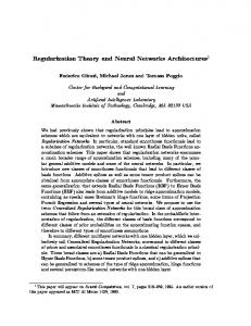
Conjugate gradient vs. Steepest descent
6- t
54L
1k
Validation (CG) Training (CG) 0 Validation (SD) Training (SD)
1
!?3w 2-
1I
OA
2000 4000 6000 8000 No. of cost and gradient func. eval.
10000
(a) Evolution of Regularization Parameters
Iteration number
dist/l997/larsen.bot.ps.Z.
Figure 1: Typical run of the K adaptation algorithm using either steepest descent (SD) or conjugate gradient (CG). Panel (a): training and validation errors in both cases. Note that CG both converges faster and yield slightly lower validation error. The total number of cost and gradient evaluation is a good measure of the total computational burden. Panel (b): evolution of the log-weight decay parameters using conjugate gradient. Most active inputs have small weight decays, while the noise inputs have higher weight decays. However, notice that the overall influence is determined by the weight decay as well as the value of the weights. The output layer weight decay is seemingly not important.
[12] R.M. Neal: Bayesian Learning for Neural Networks, New York: Springer Verlag, 1996. [13] W.H. Press, S.A. Teukolsky, W.T. Vetterling, & B.P. Flannery: Numerical Recipes in C, The Art of Scientific Computing, Cambridge, Massachusetts: Cambridge University Press, 2nd Edition, 1992. [14] Carl E. Rasmussen: Evaluation of Gaussian Processes and Other Methods for Non-Linear Regression, Ph.D. Thesis, Dept. of Computer Science, Univ. of Toronto, 1996. Available by: f t p : / / ftp.cs.toronto.edu/pub/carl/thesis.ps.gz.
[15] G.A.F. Seber & C.J. Wild: Nonlinear Regression, New York, New York: John Wiley & Sons, 1989. [16] M.P. Wand & M.C. Jones: Kernel Smoothing, New York, New York: Chapman & Hall, 1995.
[3] J.E. Dennis & R.B. Schnabel: Numerical Meth-
1204
Authorized licensed use limited to: Danmarks Tekniske Informationscenter. Downloaded on June 01,2010 at 10:53:42 UTC from IEEE Xplore. Restrictions apply.