Adaptive Rejection Sampling with fixed number of nodes

Adaptive Rejection Sampling with fixed number of nodes L. Martino? , F. Louzada?

arXiv:1509.07985v1 [stat.CO] 26 Sep 2015

?

Institute of Mathematical Sciences and Computing, Universidade de S˜ ao Paulo, S˜ ao Carlos (S˜ ao Paulo).

Abstract The adaptive rejection sampling (ARS) algorithm is a universal random generator for drawing samples efficiently from a univariate log-concave target probability density function (pdf). ARS generates independent samples from the target via rejection sampling with high acceptance rates. Indeed, ARS yields a sequence of proposal functions that converge toward the target pdf, so that the probability of accepting a sample approaches one. However, sampling from the proposal pdf becomes more computational demanding each time it is updated. In this work, we propose a novel ARS scheme, called Cheap Adaptive Rejection Sampling (CARS), where the computational effort for drawing from the proposal remains constant, decided in advance by the user. For generating a large number of desired samples, CARS is faster than ARS. Keywords: Monte Carlo methods, Rejection Sampling, Adaptive Rejection Sampling 1. Introduction Random variate generation is required in different fields and several applications (Devroye, 1986; H¨ormann et al., 2003; Robert and Casella, 2004). Rejection sampling (RS) (Robert and Casella, 2004, Chapter 2) is a universal sampling method which generates independent samples from a target probability density function (pdf). The sample is either accepted or rejected by an adequate test of the ratio of the two pdfs. However, RS needs to establish analytically a bound for the ratio of the target and proposal densities.

Preprint submitted to Elsevier

September 29, 2015

Given a target density, the adaptive rejection sampling (ARS) method (Gilks and Wild, 1992; Gilks, 1992) produces jointly both a suitable proposal pdf and the upper bound for the ratio of the target density over this proposal. Moreover, the main advantage of ARS is that ensures high acceptance rates, since ARS yields a sequence of proposal functions that actually converge toward the target pdf when the procedure is iterated. The construction of the proposal pdf is obtained by a non-parametric procedure using a set of support points (nodes), with increasing cardinality. When a sample is rejected in the RS test, it is added to the set of support points. One limitation of ARS is that it can be applied only with (univariate) log-concave target densities.1 For this reason, several extensions have been proposed (H¨ormann, 1995; Hirose and A.Todoroki, 2005; Evans and Swartz, 1998; G¨or¨ ur and Teh, 2011; Martino and M´ıguez, 2011), even mixing with MCMC techniques (Gilks et al., 1995; Martino et al., 2013, 2015a). A related RS-type method, automatic but nonadaptive, that employs a piecewise constant construction of the proposal density obtained with a pruning of the initial nodes, has been suggested in (Martino et al., 2015b). In this work, we focus on the computational cost required by ARS. The ARS algorithm obtains high acceptance rates improving the proposal function, which becomes closer and closer to target function. Hence, this enhancement of the acceptance rate is obtained building more complex proposals, which become more computational demanding. The overall time of ARS depends on both the acceptance rate and the time required for sampling from the proposal pdf. The computational cost of ARS remains bounded since the probability of updating the proposal pdf, Pt , vanishes to zero as the number of iterations t grows. However, for a finite t, there is always a positive probability Pt > 0 of improving the proposal function, producing an increase of the acceptance rate. This enhancement of the acceptance rate could not balance out the increase of the time required for drawing from the new updated proposal function. Namely, if the acceptance rate is enough close to 1, a further improvement of the proposal function could become prejudicial. Thus, we propose a novel ARS scheme, called Cheap Adaptive Rejection Sampling (CARS), employing always a fixed number of nodes, i.e., the com1

The possibility of applying ARS for drawing for multivariate densities depends on the ability of constructing a sequence of non-parametric proposal pdfs in higher dimensions. See, for instance, the piecewise constant construction in (Martino et al., 2015a) as a simpler alternative procedure.

2

putational effort required for sampling from the proposal remains constant, selected in advance by the user. The new technique is able to increase the acceptance rate on-line in the same fashion of the standard ARS method, improving adaptively the location of the support points. The configuration of the nodes converges to the best possible distribution which maximizes the acceptance rate achievable with a fixed number of support points. Clearly, the maximum obtainable acceptance rate with CARS is always smaller than 1, in general. However, for large value of required samples, the CARS algorithm is faster than ARS for generating independent samples from the target, as shown the numerical simulations. 2. Adaptive Rejection Sampling We denote the target density as π ¯ (x) = with cπ =

R X


1 1 π(x) = exp V (x) , cπ cπ

x ∈ X ⊆ R,

π(x)dx. The adaptive proposal pdf is denoted as q¯t (x) =


1 1 qt (x) = exp Wt (x) , ct cπ

R where ct = X qt (x)dx and t ∈ N. In order to apply rejection sampling (RS), it is necessary to build qt (x) as an envelope function of π(x), i.e., qt (x) ≥ π(x),

or

Wt (x) ≥ V (x),

(1)

for all x ∈ X and t ∈ N. As a consequence, it is important to observe that ct ≥ cπ ,

∀t ∈ N.

(2)

Let us assume that V (x) = log π(x) is concave, and we are able to evaluate the function V (x) and its first derivative V 0 (x).2 The adaptive rejection The evaluation of V 0 (x) is not strictly necessary, since the function qt (x) can also construct using a derivative-free procedure (e.g., see (Gilks, 1992) or the piecewise constant construction in (Martino et al., 2015a)). For the sake of simplicity, we consider the construction involving tangent lines. 2

3

sampling (ARS) technique (Gilks, 1992; Gilks and Wild, 1992) considers a set of support points at the t-th iteration, St = {s1 , s2 , . . . , smt } ⊂ X , such that s1 < . . . < smt and mt = |St |, for constructing the envelope function qt (x) in a non-parametric way. We denote as wi (x) as the straight line tangent to V (x) at si for i = 1, . . . , mt . Thus, we can build a piecewise linear function, Wt (x) = min[w1 (x), . . . , wmt (x)],

x ∈ X.

(3)

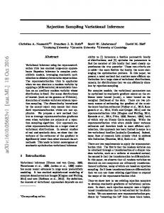
Hence, the proposal pdf defined as q¯t (x) ∝ qt (x) = exp(Wt (x)), is formed by exponential pieces in such a way that Wt (x) ≥ V (x), so that qt (x) ≥ π(x), when V (x) is concave (i.e., π(x) is log-concave). Figure 1 depicts an example of piecewise linear function Wt (x) built with mt = 3 support points. w2 (x)

w1 (x) €

Wt (x)

V (x)

w3 (x)

€

€

€

€

s1

s2

s3

Figure 1: Example of construction of the piecewise linear function Wt (x) with mt = 3 support points, such that Wt (x) ≥ V (x).

€ € € Table 1 summarizes the ARS algorithm for drawing N independent samples from π ¯ (x). At each iteration t, a sample x0 is drawn from q¯t (x) and 0) accepted with probability qπ(x 0 ) , otherwise is rejected. Note that a new point (x t is added to the support set St whenever it is rejected in the RS test improving the construction of qt (x). Clearly, denoting as T the total number of iterations of the algorithm, we have always T ≥ N since several samples are discarded.

4

Table 1: Adaptive Rejection Sampling (ARS) algorithm.

Initialization: 1. Set t = 0 and n = 0. Choose an initial set S0 = {s1 , . . . , sm0 }. Iterations (while n < N ): 2. Build the proposal qt (x), given the set of support points St = {s1 , . . . , smt }, according to Eq. (3). 3. Draw x0 ∼ q¯t (x) ∝ qt (x) and u0 ∼ U([0, 1]). 4. If u0 >

π(x0 ) , qt (x0 )

then reject x0 , update St+1 = St ∪ {x0 },

and set t = t + 1. Go back to step 2. 5. If u0 ≤

p(x0 ) , πt (x0 )

then accept x0 , setting xn = x0 .

6. Set St+1 = St , t = t + 1, n = n + 1 and return to step 2. Outputs: The N accepted samples x1 , . . . , xN . 3. Computational cost of ARS The computational cost of an ARS-type method depends on two elements: 1. The averaged number of accepted samples, i.e., the acceptance rate. 2. The computational effort required for sampling from qt (x). We desire that the acceptance rate is close to 1 and, simultaneously, that the spent time required for drawing from qt (x) is small. In general, there exists a trade-off since an increase of the acceptance rate requires the use of a more complicated proposal density qt (x). ARS is an automatic procedure which provides a possible compromise. Below, we analyze some important features of a standard ARS scheme.

5

3.1. Acceptance rate The averaged number of accepted samples, i.e., the acceptance rate, is Z π(x) cπ q¯t (x)dx = , (4) ηt = qt (x) ct that is 0 ≤ ηt ≤ 1 since ct ≥ cπ , ∀t ∈ N, by construction. Defining the L1 distance between πt (x) and p(x) as Z D(qt , π) = kqt (x) − π(x)k1 = |qt (x) − π(x)|dx, (5) X

ARS ensures that D(qt , π) → 0 when t → ∞, and as a consequence ct → cπ . Thus, ηt tends to one as t → ∞. Indeed, as ηt → 1, ARS becomes virtually an exact sampler after a some iterations. 3.2. Drawing from the proposal pdf Let us denote the exponential pieces as hi (x) = ewi (x) ,

i = 1, . . . , N,

(6)

so that qt (x) = hi (x),

for

x ∈ Ii = (ei−1 , ei ],

i = 1, . . . , N,

where ei is the intersection point between the straight lines wi (x) and wi+1 (x), for i = 2, . . . , N − 1, and e0 = −∞ and eN = +∞ (if X = R). Thus, for drawing a sample x0 from q¯t (x) = c1t qt (x), we need to: 1. Compute analytically the area Ai below each exponential piece, i.e., R Ai = Ii hi (x)dx and obtain the normalized weights Ai ρi = PN

n=1 An

where we have observed that ct =

PN

=

Ai , ct

n=1 An =

(7) R X

qt (x)dx.

2. Select an index j ∗ (namely, one piece) according to the probability mass ρi , i = 1, . . . , N .

6

3. Draw x0 from hj ∗ (x) restricted within the domain Ij ∗ = (ej ∗ −1 , ej ∗ ], and zero outside (i.e., from a truncated exponential pdf). Observe that, at step 2, a multinomial sampling is required. It is clear that the computational cost for drawing one sample from qt (x) increases as the number of pieces grows or, equivalently, the number of support points grows. Fortunately, the computational cost in ARS is automatically controlled by the algorithm, since the probability of adding a new support point Pt = 1 − η t =

1 D(qt , π), ct

(8)

tends to zero as t → ∞, since the distance in Eq. (5) vanishes to zero, i.e., D(qt , π) → 0. 4. ARS with fixed number of support points We have seen that the probability of adding a new support point Pt vanishes to zero as t → ∞. However, for a finite t, we have always a positive probability Pt > 0 of adding a new point (although small), so that a new support point could be incorporated producing an increase of the acceptance rate. After a certain iteration τ , i.e., t > τ , this improvement of the acceptance rate could not balance out the increase of the time required for drawing from the proposal, due to the addition of the new point. Namely, if the acceptance rate is enough close to 1, a further addition of a support point could slow down the algorithm, becoming prejudicial. In this work, we provide an alternative adaptive procedure for ARS, called Cheap Adaptive Rejection Sampling (CARS), which uses a fixed number of support points. When a sample is rejected, a test for swapping the rejected sample with the closest support point within St is performed, so that the total number of points remains constant. Unlike in the standard ARS method, in the new adaptive scheme the test is deterministic. The underlying idea is based on the following observation. The standard ARS algorithm yields a decreasing sequence R of normalizing constants {ct }t∈N of the proposal pdf converging to cπ = X π(x)dx, i.e., c0 ≥ c1 . . . ≥ ct . . . ≥ c∞ = cπ .

(9)

Clearly, since the acceptance rate is ηt = ccπt this means that ηt → 1. In CARS, we provide an alternative way for producing this decreasing sequence 7

of normalizing constants {ct }. Indeed, an exchange between two points is accepted if it produces a reduction in the normalizing constant of the corresponding proposal pdf. More specifically, consider the set St = {s1 , s2 , . . . , sM }, contained M support points. When a sample x0 is rejected in the RS test, the closest support point s∗ in St is obtained, i.e., s∗ = arg min |si − x0 |. si ∈St

We recall that we denote with qt (x) the proposal pdf built using St and with ct its normalizing constant. Then, we consider a new set G = St ∪ {x0 }\{s∗ },

(10)

namely, including x0 and removing s∗ . We denote with g(x) R the proposal built using the alternative set of support points G, and cg = X g(x)dx. If cg < ct , then the swap is accepted, i.e., we set St+1 = G for the next iteration, otherwise the set remains unchanged, St+1 = St . The complete algorithm is outlined in Table 2. Note that ct is always computed (in any case, for both ARS and CARS) at the step 3, for sampling from qt (x). Furthermore observe that, after the first iteration, step 2 can be skipped since the new proposal pdf qt+1 (x) has been already constructed in the previous iteration, i.e., qt+1 (x) = qt (x), or at step 4.3, i.e., qt+1 (x) = g(x). Therefore, with the CARS algorithm, we obtain again a decreasing sequence of {ct }t∈N c0 ≥ c1 . . . ≥ ct . . . ≥ c∞ , but c∞ 6= cπ so that ηt → η∞ < 1, in general. The value η∞ is the highest acceptance rate that can be obtained with M support points, given the target function π(x). Therefore, CARS yields a sequence of sets S1 , . . . , St , . . . that converges to the stationary set S∞ containing the best configuration of M support points for maximizing the acceptance rate, when the target function is π(x) and given a specific construction procedure for the proposal qt (x).3 3

The best configuration S∞ depends on the specific construction procedure employed for building the sequence of proposal functions q1 , q2 . . . , qt , . . .

8

Table 2: Cheap Adaptive Rejection Sampling (CARS) algorithm.

Initialization: 1. Set t = 0 and n = 0. Choose a value M and an initial set S0 = {s1 , . . . , sM }. Iterations (while n < N ): 2. Build the proposal qt (x), given the current set St , according to Eq. (3) or other suitable procedures. 3. Draw x0 ∼ q¯t (x) ∝ qt (x) and u0 ∼ U([0, 1]). 4. If u0 >

π(x0 ) , qt (x0 )

then reject x0 and:

4.1 Find the closest point s∗ in St , s∗ = arg min |si − x0 |. si ∈St

4.2 Build the alternative proposal g(x) based on the set of points G = St ∪ {x0 }\{s∗ } and compute cg =

R X

g(x)dx.

4.3 If cg < ct , set St+1 = G, otherwise, if cg ≥ ct , set St+1 = St . Set t = t + 1 and go back to step 2. 5. If u0 ≤

p(x0 ) , πt (x0 )

then accept x0 , setting xn = x0 .

6. Set St+1 = St , t = t + 1, n = n + 1 and return to step 2. Outputs: The N accepted samples x1 , . . . , xN . 5. Numerical simulations We consider a Gaussian density as (typical) log-concave target pdf and test both ARS and CARS. Namely, we consider   x2 π ¯ (x) ∝ π(x) = exp − 2 , x ∈ R, 2σ 9

with σ 2 = 12 . We compare ARS and CARS in terms of the time required for generating N ∈ {5000, 1000} samples. In all cases and both techniques, we consider a initial set of support points S0 = {s1 , . . . , s0 } with cardinality m0 = |S0 | ∈ {3, 5, 10} (clearly, M = m0 in CARS) where the initial points are chosen uniformly in [−2, 2] at each simulation, i.e., si ∼ U([−2, 2]).4 We run 500 independent simulations for each case and compute the required time for generating N samples (using a Matlab code), the averaged number of final support points (denote as E[mT ]) and the acceptance rate reached in the final iteration (denoted as E[ηT ]; averaged over the 500 runs), for both techniques. Table 3 shows the results. The time is normalized with respect to the time spent by ARS with N = 5000, |S0 | = 3. The results show that CARS is always faster than ARS. We can observe that both methods obtain acceptance rates close to 1. CARS reaches acceptance rates always greater of 0.87 using only 3 nodes. CARS obtains an more than 0.98 employing only 10 nodes and after generating N = 5000 independent samples. Fig. 2 depicts the wasted time, the final acceptance rate and the final number of nodes, as function of number N of generated samples. We can observe that CARS is significantly faster than ARS when N grows, owing to ARS yields a sensible increase of the number of support points that corresponds to an infinitesimal increase of the acceptance rate, whereas CARS the number of nodes remains constant. Figure 3 shows a sequence of proposal pdfs constructed by CARS, using 3 nodes and starting with S0 = {−1.5, −1, 1.8}. The L1 distance D(qt , π) is reduced progressively and the acceptance rate improved. The final set of support point is St = {−1.0261, −0.0173, 1.0305}, close to the optimal one S∞ = {−1, 0, 1}. 6. Acknowledgements This work has been supported by the Grant 2014/23160-6 of S˜ao Paulo Research Foundation (FAPESP) and by the Grant 305361/2013-3 of National Council for Scientific and Technological Development (CNPq). References L. Devroye. Non-Uniform Random Variate Generation. Springer, 1986. 4

Clearly, the configurations of either all negative or all positive are discarded since they yield improper proposal pdf by construction.

10

Table 3: Results as function of the desired number of samples N and the cardinality |S0 | of the initial set of support points S0 . We show the normalized spent time, the averaged final number of support points, E[mT ], and the averaged final acceptance rate, E[ηT ]. Scheme

N

ARS

5000

CARS

5000

ARS

10000

CARS

10000

ARS

50000

CARS

50000

|S0 | = 3 Time=1 E[ηT ] = 0.9942 E[mT ] = 32.36 Time=0.9599 E[ηT ] = 0.8721 E[mT ] = M = 3 Time=2.2843 E[ηT ] = 0.9963 E[mT ] = 40.60 Time=1.9716 E[ηT ] = 0.8784 E[mT ] = M = 3 Time=11.2196 E[ηT ] = 0.9987 E[mT ] = 68.63 Time=8.7756 E[ηT ] = 0.8855 E[mT ] = M = 3

|S0 | = 5 Time=0.9709 E[ηT ] = 0.9945 E[mT ] = 32.69 Time=0.9477 E[ηT ] = 0.9224 E[mT ] = M = 5 Time=1.9862 E[ηT ] = 0.9964 E[mT ] = 41.09 Time=1.7311 E[ηT ] = 0.9350 E[mT ] = M = 5 Time=11.2887 E[ηT ] = 0.9987 E[mT ] = 69.56 Time=8.4322 E[ηT ] = 0.9540 E[mT ] = M = 5

|S0 | = 10 Time=0.9801 E[ηT ] = 0.9952 E[mT ] = 34.17 Time=0.9694 E[ηT ] = 0.9556 E[mT ] = M = 10 Time=1.9983 E[ηT ] = 0.9968 E[mT ] = 42.16 Time=1.8969 E[ηT ] = 0.9631 E[mT ] = M = 10 Time=11.7599 E[ηT ] = 0.9988 E[mT ] = 70.09 Time=9.0704 E[ηT ] = 0.9861 E[mT ] = M = 10

W. H¨ormann, J. Leydold, and G. Derflinger. Automatic nonuniform random variate generation. Springer, 2003. C. P. Robert and G. Casella. Monte Carlo Statistical Methods. Springer, 2004. W. R. Gilks and P. Wild. Adaptive Rejection Sampling for Gibbs Sampling. Applied Statistics, 41(2):337–348, 1992. W. R. Gilks. Derivative-free Adaptive Rejection Sampling for Gibbs Sampling. Bayesian Statistics, 4:641–649, 1992. L. Martino, J. Read, and D. Luengo. Independent doubly adaptive rejection Metropolis sampling within Gibbs sampling. IEEE Transactions on Signal Processing, 63(12):3123–3138, 2015a.

11

Required Time 12 10

Final Acceptance Rate

ARS CARS

Final number of support points

1

60

0.8

40

ARS CARS

8 6 4

20

2 0

ARS CARS

0.6 1

2

3 N

(a)

4

5 4 x 10

1

2

3 N

(b)

4

5 4 x 10

0

1

2

3 N

4

5 4 x 10

(c)

Figure 2: (a) Spent time, (b) final acceptance rate, and (c) final number of support points, as function of the number N of drawn samples, for ARS (squares) and CARS (triangles).

W. H¨ormann. A rejection technique for sampling from T-concave distributions. ACM Transactions on Mathematical Software, 21(2):182–193, 1995. H. Hirose and A.Todoroki. Random number generation for the generalized normal distribution using the modified adaptive rejection method. International Information Institute, 8(6):829–836, March 2005. M. Evans and T. Swartz. Random variate generation using concavity properties of transformed densities. Journal of Computational and Graphical Statistics, 7(4):514–528, 1998. Dilan G¨or¨ ur and Yee Whye Teh. Concave convex adaptive rejection sampling. Journal of Computational and Graphical Statistics, 20(3):670–691, September 2011. L. Martino and J. M´ıguez. A generalization of the adaptive rejection sampling algorithm. Statistics and Computing, 21(4):633–647, October 2011. W. R. Gilks, N. G. Best, and K. K. C. Tan. Adaptive Rejection Metropolis Sampling within Gibbs Sampling. Applied Statistics, 44(4):455–472, 1995. L. Martino, R. Casarin, F. Leisen, and D. Luengo. Adaptive Sticky Generalized Metropolis. arXiv:1308.3779, 2013. L. Martino, H. Yang, D. Luengo, J. Kanniainen, and J. Corander. A fast universal self-tuned sampler within Gibbs sampling. (in press) Digital Signal Processing, 2015b. 12

Initial proposal pdf q0(x)

8

Proposal after generating N=100 samples (t≥ N)

1.5

π(x) si

π(x) si

6

q (x)

qt(x)

1

t

4 0.5 2 0 −4

−2

0

2

0 −4

4

−2

0

(a)

2

4

(b) Proposal after generating N=10000 samples (t≥ N)

1.5

π(x) si q (x) t

1

0.5

0 −4

−2

0

2

4

(c) Figure 3: Example of sequence of proposal pdfs obtained by CARS, starting with S0 = {−1.5, −1, 1.8}. We can observe that the L1 distance D(qt , π) is reduced progressively. The proposal function qt (x) is depicted with dashed line, the target function π(x) with solid line and the support points with circles. The configuration of the nodes in figure (c) is St = {−1.0261, −0.0173, 1.0305} with t ≥ N = 104 . The optimal configuration with 3
2 nodes and π(x) = exp −x is S∞ = {−1, 0, 1}.

13