This paper proposes a multi-dimensional adaptive sampling algorithm for rendering applications. .... path space, which is transformed to a D-dimensional unit.
Fifth Hungarian Conference on Computer Graphics and Geometry, Budapest, 2010
Adaptive Sampling with Error Control László Szécsi1 , László Szirmay-Kalos1 , and Murat Kurt2 1:
BME IIT, Hungary, 2 : International Computer Institute, Ege University, Turkey
Abstract This paper proposes a multi-dimensional adaptive sampling algorithm for rendering applications. Unlike importance sampling, adaptive sampling does not try to mimic the integrand with analytically integrable and invertible densities, but approximates the integrand with analytically integrable functions, thus it is more appropriate for complex integrands, which correspond to difficult lighting conditions and sophisticated BRDF models. We develop an adaptation scheme that is based on ray-differentials and does not require neighbor finding and complex data structures in higher dimensions. As a side result of the adaptation criterion, the algorithm also provides error estimates, which are essential in predictive rendering applications.
1. Introduction Rendering is mathematically equivalent to the evaluation of high-dimensional integrals. In order to avoid the curse of dimensionality, Monte Carlo or quasi-Monte Carlo quadratures are applied, which take discrete samples and approximate the integral as the weighted sum of the integrand values in these samples. The challenge of these methods is to find a sampling strategy that generates a small number of samples providing an accurate quadrature. Importance sampling would mimic the integrand with the density of the samples. However, finding a proper density function and generating samples with its distribution are non-trivial tasks. There are two fundamentally different approaches to generating samples with a probability density. The inversion method maps uniformly distributed samples with the inverse of the cumulative probability distribution of the desired density. However, this requires that the density is integrable and its integral is analytically invertible. The integrand of the rendering equation is a product of BRDFs and cosine factors of multiple reflections, and of the incident radiance at the end of a path. Due to the imposed requirements, importance sampling can take into account only a single factor of this product form integral, and even the single factor is just approximately mimicked except for some very simple BRDF models. Rejection sampling based techniques, on the other hand, do not impose such requirements on the density. However, rejection sampling may ignore many, already generated samples, which may lead to unpredictable
performance degradation. Rejection sampling inspired many sampling methods 5, 28, 1, 20, 22, 27 . We note that in the context of Metropolis sampling there have been proposals to exploit even the rejected samples having re-weighted them 30, 10, 17, 13 . Hierarchical sampling strategies attack product form integrands by mimicking just one factor initially, then improving the sample distribution in the second step either by making the sampling distribution more proportional to the integrand 5, 28, 6, 7, 22 or by making the empirical distribution of the samples closer to the continuous sample distribution 1, 20, 27 . An alternative method of finding samples for integral quadratures is adaptive sampling that uses the samples to define an approximation of the integrand, which is then analytically integrated. Adaptation is guided by the statistical analysis of the samples in the sub-domains. Should the variance of the integrand in a sub-domain be high, the sub-domain is broken down to smaller sub-domains. Adaptive sampling does not pay attention to the placement of the samples in the sub-domains. However, placing samples in a sub-domain without considering the distribution of samples in neighboring sub-domains will result in very uneven distribution in higher dimensional spaces. On the other hand, variance calculation needs neighbors finding, which gets also more difficult in higher dimensions. Thus, adaptive sampling usually suffers from the curse of dimensionality. The VEGAS method 18 is an adaptive Monte-Carlo technique that generates a probability density for importance
Szécsi, Szirmay-Kalos, Kurt / Adaptive Sampling with Error Control
sampling automatically and in a separable form. The reason of the requirement of separability is that probability densities are computed from and stored in histogram tables and s number of 1-dimensional tables need much less storage space than a single s-dimensional table. This paper proposes a multi-dimensional adaptive sampling scheme, which: • works with vector valued functions as well and does not require the introduction of simple scalar valued importance unlike in importance sampling algorithms, • is simple to implement even in higher dimensions, • has small additional overhead both in terms of storage and computation, because it does not require complex data structures or neighborhood searches as other adaptive algorithms, • provides consistent, deterministic estimates with small and predictable quadrature error (the term unbiasedness is not applicable for deterministic sampling algorithms).
2. Previous work Adaptive sampling: Adaptive sampling uses samples to approximate the integrand, thus concentrates samples where the integrand changes significantly. The targeted approximation is usually piece-wise constant or piece-wise linear 14 . Image space adaptive sampling was used even in the first ray tracer 31 , and has been improved by randomization 4 and by the application of information theory tools 21 . Adaptive sampling methods should decompose the sampling domain, which is straightforward in 2D but needs special data structures like the kd-tree in higher dimensions 11 . Ray- and path-differentials: A ray-differential means the derivative of the contribution of a path with respect to some variable defining this path. Igehy introduced ray-differentials with respect to screen-space coordinates 12 . Ray-differentials were used in filtering applications where the differentials define the footprint of the samples, i.e. the domain the filter. Suykens 25 generalized this idea for arbitrary sampling parameters defining the path. Photon differentials 24 also use this concept to enhance radiance estimates in photon mapping. We note that unlike these techniques, we do not use path-differentials in this paper for setting up filters, but to guide the sampling process. Error estimation in rendering: In predictive rendering we need not only an estimate of the image, but also error bounds describing the accuracy of the method 29 . Unfortunately, the computation of the error of a rendering algorithm is even more complex than producing the image 2 . Error analysis was proposed in the context of finite-element based radiosity methods 19, 3, 4, 23 . For Monte-Carlo methods, we can use the statistics of the samples to estimate the variance of the estimator. For deterministic approaches, in theory, the KoksmaHlawka inequality could be used. However, due to the in-
finite variation of the typical integrands in rendering, this provides useful bounds only in exceptional cases 26 . 3. Proposed sampling scheme For the sake of notational simplicity, let us consider first a 1D integral of a possibly vector valued integrand f (t) in the domain of [0, 1]. Suppose that the integration domain is decomposed to intervals ∆(1) , ∆(2) , . . . , ∆(M) and one sample point t (i) is selected in each of them. The integral is estimated in the following way: ∫1
f (t)dt ≈
M
∑ f (t (i) )∆(i) .
(1)
i=1
0
f’(t2)∆2
f’(t3)∆3
f’(t1)∆1
t1
∆1
t2
∆2
t3 ∆4
Figure 1: The error of adaptive sampling is the total area of triangles of bases ∆i and heights that are proportional to ∆i and to the derivative of integrand f . Looking at Figure 1, we can conclude that the error of the integral is the sum of small triangles in between the integrand and its piece-wise constant approximation, which can be expressed as follows if derivative f ′ exists: ( )2 ∫1 M M ∆(i) f (t)dt − ∑ f (t (i) )∆(i) ≈ ∑ | f ′ (t (i) )| . (2) 2 0 i=1 i=1 (i) We minimize the error with the constraint ∑M i=1 ∆ = 1 using the Lagrange multiplier method. The target function that also includes the constraint is ( )2 ( ) M ∆(i) ′ (i) | f (t )| − λ ∑ ∆(i) − 1 . ∑ 2 i=1
Computing the partial derivatives with respect to ∆(i) and making it equal to zero, we obtain: | f ′ (t (i) )|∆(i) = λ, i = 1, 2, . . . , M, thus, the variation in all sub-domains should be equal, i.e. the sampling scheme should concentrate samples where the integrand changes quickly. 3.1. Extension to integrands typical in rendering The integrand of rendering is defined in a high-dimensional path space, which is transformed to a D-dimensional unit cube U . A point in the unit cube is denoted by u =
Szécsi, Szirmay-Kalos, Kurt / Adaptive Sampling with Error Control
(u1 , . . . , uD ). The integrand is high-dimensional, can only be point sampled, but together with point sampling, its derivative can also be obtained according to the concept of raydifferentials. Adaptive sampling should decompose the integration domain, i.e. the unit cube to M sub-domains. Sub-domain i has (i) (i) edge lengths ∆1 , . . . , ∆D and volume (i)
(i)
∆(i) = ∆1 · . . . · ∆D . Each sub-domain contains a single sample u(i) from which the integral is estimated as: ∫
M
F(u)du ≈
∑ F(u(i) )∆(i) .
(3)
i=1
U
In order to find the error of this multi-dimensional integral, we approximate the integrand by the first-order Taylor series in each sub-domain: F(u) ≈ F(ui ) +
∂F(u(i) ) (i) (ud − ud ). ∂u d d=1 D
∑
Substituting this approximation into the quadrature error, we get: ∫ (i) ∆(i) M M D ∂F(u ) d (i) (i) (i) F(u)du − ∑ F(u )∆ ≈ ∑ ∑ ∆ . i=1 d=1 ∂ud 2 i=1 U
We work with the Halton series, but other low discrepancy series, such as the Sobol series or (t, m, s)-nets with t = 0 could be used as well 15 . For the 1D Halton sequence in base B, the elemental interval property means that the sequence will visit all intervals of length [kB−R , (k + 1)B−R ) before putting a new point in an interval already visited. As the sequence is generated, the algorithm produces a single point in each interval of length B−1 , then in each interval of length B−2 , etc. For a D-dimensional sequence of relative prime bases B1 , . . . , BD , this property means that the sequence will insert a sample in each cell −RD 1 1 D [k1 B−R , (k1 + 1)B−R ) × . . . × [kD B−R D , (kD + 1)BD ) 1 1
before placing a second sample in any of these cells. The elemental interval property thus implicitly defines an automatically refined sub-domain structure, which can also be exploited in adaptive sampling. If we decide to subdivide the sub-domain of sample i along coordinate axis d, then the following new samples must be generated: D
D
D
d=1
d=1
d=1
i + ∏ BRd d , i + 2 ∏ BRd d , . . . , (Bd − 1) ∏ BRd d .
(4)
We minimize this error by finding the sub-domain sizes (i) ∆d satisfying the constraints that sub-domains are disjunct and their union is the original unit cube. If sub-domain ∆(i) is subdivided along axis d, the error is reduced proportionally by (i) ∂F(u ) (i) (i) (i) εd = ∆ ∆ . ∂ud d To maximize the error reduction, that sub-domain and dimension should be selected for subdivision where this product is maximum. As each sub-domain stores a single sample, the reduced error can also be assigned to the samples. Samples are generated one-by-one. When we are at sample ui , the integrand as well its partial derivatives are computed, and each sample is given the vector of possible error reductions: [ ] (i) (i) ε(i) = ε1 , . . . , εD . The maximum error reduction with respect to all samples and dimensions tells us which sub-domain should be subdivided and also specifies the axis of the subdivision. The subdomain is subdivided generating new samples in the neighborhood of the sample associated with the subdivided cell. 3.2. Sample generation and sub-domain subdivision In order to explore the integration domain and establish the subdivision scheme, we take a low-discrepancy series 16, 9 .
2 1
5
2 1
5
2 4
1
1
3 1 R1=0 R2=0 Bases: B1=2, B2=3
1 1 2 R1=1 R2=0
3
1 1 1 3 5 R1=1 R2=1
1 2
1
2
1 3 5 2 4 R1=1 R2=1
R1=2 R2=0
Figure 2: Evolution of samples and their corresponding subdomains in 2D with a Halton sequence of bases B1 = 2 and B2 = 3. In Figure 2 we show the evolution of the cell structure in 2D as new samples are introduced. First, we have a single sample j = 1 in a cell of volume 1 (R1 = 0, R2 = 0). Then, this cell is subdivided along the first axis where the basis is 1 −R2 B1 = 2, generating a new sample j = 1 + B−R B2 = 2. 1 Simultaneously, the size of the cell is reduced to half (R1 = 1, R2 = 0). In the third step, the cell of sample j = 1 is subdivided again, but now along the second axis. This hap1 −R2 pens by producing new samples j = 1 + B−R B2 = 3 and 1 −R1 −R2 j = 1 + 2B1 B2 = 5, with cell sizes as (R1 = 1, R2 = 1). Finally the cell of sample j = 2 is subdivided into two parts. The sampling process can be visualized as a tree (Figure 2) where upper level nodes are the subdivided subdomains, and leaves are the cells containing exactly one
Szécsi, Szirmay-Kalos, Kurt / Adaptive Sampling with Error Control
sample. The number of children of a node equals to the corresponding the prime basis number of the Halton sequence. Although only leaves are relevant for the approximation, it is worth maintaining the complete tree structure since it also helps to find that leaf which should be subdivided to reduce the error most effectively. In upper level nodes, we maintain the maximum error of its children. The generation of a new sample is the traversal of this tree. When traversing a node, we continue descending into the direction of the child with maximum error. When we arrive at a leaf, the dimension which reduces the error the most is subdivided and the leaf becomes a node with children including the original sample and the new samples. While ascending on the tree, the maximum error of the new nodes are propagated. The recursive function implementing this scheme gets a node c. Calling this function with the root node, it generates a new sample that reduces the integration error the most, and updates the complete tree as well: Process(c) if (c is a leaf) i = sample id of this leaf (R1 , . . . , RD ) = subdivision levels of this node (ε1 , . . . , εD ) = errors of this node Find the dimension d of the highest error εd for k = 1 to Bd − 1 do Rd Generate sample with id j = i + k ∏D d=1 Bd Compute F(u j ) and the partial derivatives Add sample j as child to node c endfor Update subdivision levels in sample i Update error in sample i Add sample i as child to node c ε(c) = maximum error of the children else Find the child node cfirst with maximum error Find the second largest error εsecond εc = max( Process(cfirst ), εsecond ) endif return ε(c) end
This algorithm works in arbitrary dimensions. In order to use the method, first we have to map the integration problem to the unit cube, and have to establish the formulae for computing the derivatives. This seems complicated, but in fact, it is quite simple. When we have the program of evaluating the integrand, the derivatives can be obtained by simply deriving the program code. In the following section, we discuss a simple application of the method for environment mapping. 3.3. Robustness issues So far we assumed that the derivative exists and is an appropriate measure for the change of the function in a subdomain. This is untrue where the function has a discontinuity
or when the sub-domain is large. From another point of view, a consistent estimator should decompose a sub-domain even if the derivative is zero at the examined sample when the number of samples goes to infinity. To obtain this behavior, a positive constant is added to the derivative before the error is computed. This constant is reduced as size of the sub-domain gets smaller, corresponding to the fact that for smaller sub-domains the derivative becomes a more reliable measure of the change of a function. Note also that the derivative does not exist where the integrand is discontinuous. This is typically the case when the integrand includes the visibility factor. Ignoring the visibility factor in the derivative computation, we can still apply the method since we use the derivatives only to decide the “optimal” decomposition of the integration domain, and not directly for the estimation of the integral. If the decomposition is not “optimal” due to the ignored factors, the method will still converge to the real value as more samples are introduced, but the convergence will be slower. In theory, it would be possible to replace the product of the derivative by more general estimates of the integration error, but they also have added cost. The proposed method uses the Halton sequence which can fill D-dimensional spaces uniformly with O(logD N/N) discrepancy. However, we cannot claim that our method remains similarly stable in very high dimensions. The problem is the index generation needed to find additional samples in the neighborhood of a given sample, can result in fast growing sequences 15 . So we propose application fields where the dimension of the integration domain is moderate. 4. Application to environment mapping Environment mapping point ⃗x as L(⃗x,⃗ω) =
∫
8
computes the reflected radiance of
Lenv (⃗ω′ ) fr (⃗ω′ ,⃗x,⃗ω) cos θ⃗′x v(⃗x,⃗ω′ )dω′ ,
Ω
where Ω is the set of all directions, Lenv (⃗ω′ ) is the radiance of the environment map at illumination direction ⃗ω′ , fr is the BRDF, θ⃗′x is the angle between the illumination direction and the surface normal at shaded point ⃗x, and v(⃗x,⃗ω′ ) is the indicator function checking whether no virtual object is seen from ⃗x at direction ⃗ω′ , so environment lighting can take effect. We suppose that the BRDF and the environment lighting are available in analytic forms. In order to transform the integration domain, i.e. the set of illumination directions, to a unit square u1 , u2 ∈ [0, 1], we find a parametrization ⃗ω′ (u1 , u2 ). We shall consider different options for this parametrization, including a global parametrization that is independent of the surface normal of the shaded point, and BRDF based parametrizations where the Jacobi determinant of the mapping compensates the variation of the BRDF and the cosine factor.
Szécsi, Szirmay-Kalos, Kurt / Adaptive Sampling with Error Control
The integral of the reflected radiance can also be evaluated in parameter space: L(⃗x,⃗ω) =
∫1 ∫1
Lenv (⃗ω′ (u1 , u2 ))R(u1 , u2 )v(⃗x,⃗ω′ (u1 , u2 ))du1 du2 .
0 0
where R(u1 , u2 ) = fr (⃗ω′ (u1 , u2 ),⃗x,⃗ω) cos θ⃗′x (u1 , u2 )
∂ω ∂u1 ∂u2
is the reflection factor defined by the product of the BRDF, the cosine of the angle between the surface normal and the incident direction, and also the Jacobi determinant of the parametrization. The derivatives of the integrand F = Lenv · R · v of environment mapping are (d = 1, 2): ∂F ∂Lenv ∂R = Rv + Lenv v. ∂ud ∂ud ∂ud Thus, we need to evaluate the derivative of the reflection factor and of environment lighting. The derivative computation is presented in the appendix. The visibility factor is piecewise constant, so its derivative would be zero. 5. Results The environment mapping algorithm has been implemented using the Direct3D 9 framework and run on an nVidia GeForce 8800 GFX GPU. In environment mapping, adaptive sampling generates points in a unit square according to the product form integrand Lenv (⃗ω′ (u1 , u2 )) fr (⃗ω′ (u1 , u2 ),⃗x,⃗ω) cos θ⃗′x (u1 , u2 )
∂ω ∂u1 ∂u2
that includes the environment illumination, the cosine weighted BRDF and the Jacobi determinant of the mapping.
In Figure 4 we compare the adaptive sampling scheme involving global parametrization and diffuse BRDF parametrization to classical BRDF sampling. The proposed adaptive scheme has significantly reduced the noise. BRDF parametrization is better than global parametrization as it automatically ignores that part of the integration domain where the cosine term would be zero. Finally in the bottom row of Figure 4 we demonstrate the adaptive sampling approach in specular surface rendering. This figure compares classical BRDF sampling, adaptive sampling with global parametrization, and adaptive sampling with Phong parametrization. 6. Conclusions This paper proposed an adaptive sampling scheme based on the elemental interval property of low-discrepancy series and the derivatives of the integrand at the samples. The derivatives provide additional information to the sampling process, which can place samples where they are really needed. The low-discrepancy series not only distributes samples globally, but it also helps refining the sample structure locally without neighborhood searches. Having generated the samples and evaluated the integral, we have all information needed to evaluate equation (4), which provides error bounds for the estimate. Such bounds are badly needed in predictive rendering applications. Acknowledgement This work has been supported by the National Office for Research and Technology and OTKA K-719922 (Hungary). Appendix: Derivative computation 6.1. Global parametrization In the case of global parametrization the unit square is mapped to the set of directions independently of the local orientation of the surface. The incident direction is obtained in spherical coordinates ϕ = 2πu1 , θ = πu2 , which are converted to Cartesian coordinates of the system defined by basis vectors ⃗i, ⃗j,⃗k: ⃗ω′ (u1 , u2 ) = ⃗i cos(2πu1 ) sin(πu2 ) + ⃗j sin(2πu1 ) sin(πu2 ) +⃗k cos(πu2 ).
Figure 3: Samples generated with BRDF parametrization displayed over the transformed integrand which simplifies to Lenv (⃗ω′ (u1 , u2 )). In Figure 3 we depicted the samples assigned to a single shaded point. Samples and the transformed integrand are shown in parameter space. Note that the proposed adaptive sampling scheme places samples at regions where the illumination changes quickly and also takes care of the stratification of the samples.
The derivatives of the incident direction are as follows: ∂⃗ω′ = −2π⃗i sin(2πu1 ) sin(πu2 ) + 2π⃗j cos(2πu1 ) sin(πu2 ), ∂u1 ∂⃗ω′ = π⃗i sin(2πu1 ) cos(πu2 )+π⃗j cos(2πu1 ) cos(πu2 )−π⃗k sin(πu2 ). ∂u2 (5) The Jacobi determinant of the global parametrization is ∂ω = 2π2 sin θ = 2π2 sin(πu2 ). ∂u1 ∂u2
Szécsi, Szirmay-Kalos, Kurt / Adaptive Sampling with Error Control
BRDF sampling
Adaptive sampling global parametrization
Adaptive sampling BRDF parametrization
Figure 4: Diffuse objects (upper and middle row) and specular objects (bottom row) rendered with BRDF sampling, adaptive sampling with global parametrization, and adaptive sampling with diffuse BRDF parametrization.
6.2. Diffuse BRDF parametrization
6.3. Specular BRDF parametrization
We can also use the parametrization developed for BRDF sampling. The illumination direction is generated in the tangent space of shaded point ⃗x, defined by surface normal ⃗N⃗x , tangent ⃗T⃗x and binormal ⃗B⃗x , and it should mimic the cosine distribution: √ √ √ ⃗ω′ = ⃗T⃗x cos(2πu1 ) u2 + ⃗B⃗x sin(2πu1 ) u2 + ⃗N⃗x 1 − u2 .
In case of a Phong BRDF, the direction is generated in reflection space defined by the reflection direction
The derivatives are: ∂⃗ω′ √ √ = −2π⃗T⃗x sin(2πu1 ) u2 + 2π⃗B⃗x cos(2πu1 ) u2 , ∂u1 1 ∂⃗ω′ ⃗ cos(2πu1 ) ⃗ sin(2πu1 ) ⃗ = T⃗x + B⃗x − N⃗x √ . √ √ ∂u2 2 u2 2 u2 2 1 − u2 The Jacobi determinant compensates the cosine term: ∂ω π π = =√ . ∂u1 ∂u2 cos θ⃗x 1 − u2
⃗ωr = 2⃗N⃗x (⃗N⃗x ·⃗ω) −⃗ω and two other orthonormal vectors ⃗Tr and ⃗Br that are perpendicular to ⃗ωr . The mapping should follow the (⃗ωr ·⃗ω′ )n function: √ 2 ⃗ω′ (u1 , u2 ) = ⃗Tr cos(2πu1 ) 1 − (1 − u2 ) n+1 + √ 2 1 ⃗Br sin(2πu1 ) 1 − (1 − u2 ) n+1 +⃗ωr (1 − u2 ) n+1 .
(6)
The derivatives are obtained as:
√ 2 ∂⃗ω′ = −2π⃗Tr sin(2πu1 ) 1 − (1 − u2 ) n+1 + ∂u1 √ 2 2π⃗Br cos(2πu1 ) 1 − (1 − u2 ) n+1 .
Szécsi, Szirmay-Kalos, Kurt / Adaptive Sampling with Error Control ∂⃗ω′ ⃗ = Tr cos(2πu1 ) ∂u2
n−1
u n+1 √ 2 + 2 (n + 1) 1 − (1 − u2 ) n+1
6.5.1. Simple sky illumination For example, a sky illumination with the Sun at direction ⃗ωsun can be expressed as Lenv (⃗ω′ ) = Lsky + Lsun (⃗ω′ ·⃗ωsun )s
n−1
⃗Br sin(2πu1 )
u2n+1
1
√ −⃗ωr n . 2 (n + 1)(1 − u2 ) n+1 (n + 1) 1 − (1 − u2 ) n+1 (7)
The Jacobi determinant of the mapping is ∂ω 2π 2π = = n . ∂u1 ∂u2 (n + 1)(⃗ωr ·⃗ω′ )n (n + 1)(1 − u2 ) n+1
where Lsky and Lsun are the sky and sun radiances, respectively, and s is the exponent describing the directional fall-off of the sun radiance. With this environment radiance, the derivatives of the environment lighting are (d = 1, 2): ( ′ ) ∂Lenv ∂⃗ω = sLsun (⃗ω′ ·⃗ωsun )s−1 ·⃗ωsun . ∂ud ∂ud
6.5.2. Texture based environment lighting 6.4. Derivatives of the reflection factor The reflection factor includes the Jacobi determinant of the mapping, so it must be discussed taking into account the parametrization. If we use diffuse BRDF parametrization for a diffuse surface, the Jacobi determinant will compensate the cosine term, making the reflection factor constant, and consequently its derivative equal to zero. Similarly, the specular BRDF parametrization of a specular surface also results in a zero derivative. For more complex BRDFs that have no exact importance sampling, we can still use BRDF parametrization of a similar BRDF, for example, that of the diffuse or the Phong solutions. Of course, their Jacobi determinants will not fully eliminate the BRDF and the cosine term, so we have some non-constant function that needs to be derived. Let us now consider global parametrization, where the Jacobi determinant is 2π2 sin πu2 . If the material is diffuse with diffuse reflectivity kdif , and the surface normal at the shaded point ⃗x is ⃗N⃗x , the partial derivatives of the reflection factor including the BRDF, the cosine term, and the Jacobi determinant, are (d = 1, 2): ( ′ ) ∂R ∂⃗ω = 2π2 kdif · N⃗x sin(πu2 ). ∂u1 ∂u1 ∂R = 2π2 kdif ∂u2
((
) ) ∂⃗ω′ · N⃗x sin(πu2 ) + π(⃗ω′ · ⃗N⃗x ) cos(πu2 ) . ∂u2
if ⃗ω′ · ⃗N⃗x ≥ 0 and zero otherwise. The derivative of the incident direction is given in equation (5). The derivatives can also be computed for specular BRDFs, for example, for the Phong BRDF: ( )n R = 2π2 kspec ⃗ω′ ·⃗ωr sin(πu2 ) where kspec is the specular reflectivity. Applying the rules of derivation systematically, we get: ) ( ( )n−1 ∂⃗ω′ ∂R = 2π2 nkspec ⃗ω′ ·⃗ωr ·⃗ωr sin(πu2 ). ∂u1 ∂u1 )n−1 ( ∂R = 2π2 nkspec ⃗ω′ ·⃗ωr ∂u2
(
) ∂⃗ω′ ·⃗ωr sin(πu2 )+ ∂ud
)n ( 2π3 kspec ⃗ω′ ·⃗ωr cos(πu2 ).
If the environment lighting is defined by a texture map, we first project it into a spherical harmonics basis: env 0 Lenv (⃗ω′ ) = ∑ Ll0 Yl (cos θ)+ l
−l
∑ ∑
l m=−1
l
env m env m Llm Yl (cos θ, sin(−mϕ)) + ∑ ∑ Llm Yl (cos θ, cos(mϕ)),
where Ylm
l m=l
are the spherical harmonics basis functions.
Global spherical angles ϕ and θ can be expressed as y x , sin ϕ = √ . cos θ = z, cos ϕ = √ 1 − z2 1 − z2 where x, y, z are the components of the incident direction vector ⃗ω′ (u1 , u2 ) = (x(u1 , u2 ), y(u1 , u2 ), z(u1 , u2 )). The derivatives of the environment requires the derivatives of the spherical basis functions. In practice the number of bands l is quite small, thus it is worth pre-computing these basis functions in algebraic form by hand. The first 9 spherical basis functions are obtained as: Y00 = 0.282095 Y1−1 = 0.488603y Y10 = 0.488603z Y11 −2 Y2 Y2−1 Y20 Y21 Y22
= 0.488603x = 1.092548xy = 1.092548yz = 0.315392(3z2 − 1) = 1.092548xz = 0.546274(x2 − y2 )
The derivatives with respect to ud (d = 1, 2) of the basis functions can be obtained by a direct derivation of the formulae: ∂Y00 = 0 ∂ud ∂Y1−1 ∂y = 0.488603 ∂ud ∂ud
6.5. Derivatives of the environment lighting
∂Y10 ∂z = 0.488603 ∂ud ∂ud
The environment lighting may be defined analytically or by a texture map.
∂Y11 ∂x = 0.488603 ∂ud ∂ud
Szécsi, Szirmay-Kalos, Kurt / Adaptive Sampling with Error Control ∂Y2−2 = 1.092548 ∂ud
(
∂x ∂x y+x ∂ud ∂ud
)
14.
A. Keller. Hierarchical Monte Carlo image synthesis. Mathematics and Computers in Simulation, 55(1–3):79–92, 2001.
15.
A. Keller. Myths of computer graphics. In H. Niederreiter and D. Talay, editors, Monte Carlo and Quasi-Monte Carlo Methods 2004, pages 217–243, Berlin, 2006. Springer-Verlag.
16.
T. Kollig and A. Keller. Efficient multidimensional sampling. Computer Graphics Forum, 21(3):557–563, 2002.
17.
Y.-C. Lai, S. Fan, S. Chenney, and C. Dyer. Photorealistic image rendering with Population Monte Carlo energy redistribution. In Eurographics Symposium on Rendering, pages 287–296, 2007.
18.
S. Agarwal, R. Ramamoorthi, S. Belongie, and H. W. Jensen. Structured importance sampling of environment maps. ACM Trans. Graph., 22(3):605–612, 2003.
G. P. Lepage. An adaptive multidimensional integration program. Technical Report CLNS-80/447, Cornell University, 1980.
19.
J. Arvo, K. Torrance, and B. Smits. A framework for the analysis of error in global illumination algorithms. SIGGRAPH ’94 Proceedings, pages 75–84, 1994.
D. Lischinski, B. Smits, and D.P. Greenberg. Bounds and error estimates for radiosity. In Computer Graphics Proceedings, pages 67–75, 1994.
20.
V. Ostromoukhov, C. Donohue, and P-M. Jodoin. Fast hierarchical importance sampling with blue noise properties. ACM Transactions on Graphics, 23(3):488–498, 2004.
21.
J. Rigau, M. Feixas, and M. Sbert. Refinement criteria based on f-divergences. In EGRW ’03, pages 260–269, 2003.
22.
F. Rousselle, P. Clarberg, L. Leblanc, V. Ostromoukhov, and P. Poulin. Efficient product sampling using hierarchical thresholding. In Computer Graphics International 2008, pages 465– 474, 2008.
23.
M. Sbert. Error and complexity of random walk Monte-Carlo radiosity. IEEE Transactions on Visualization and Computer Graphics, 3(1), 1997.
24.
L. Schjoth, J. R. Frisvad, K. Erleben, and J. Sporring. Photon differentials. In GRAPHITE ’07, pages 179–186, 2007.
25.
F. Suykens and Y. D. Willems. Path differentials and applications. In In Rendering Techniques 2001, pages 257–268. 2001.
26.
K. Dmitriev, S. Brabec, K. Myszkowski, and H.-P. Seidel. Interactive global illumination using selective photon tracing. In EGRW ’02, pages 25–36, 2002.
L. Szirmay-Kalos, T. Fóris, L. Neumann, and B. Csébfalvi. An analysis to quasi-Monte Carlo integration applied to the transillumination radiosity method. Computer Graphics Forum (Eurographics’97), 16(3):271–281, 1997.
27.
10. A. Guillin, J. M. Marin, and C. P. Robert. Population Monte Carlo. Journal of Computational and Graphical Statistics, 13:907–929, 2004.
L. Szirmay-Kalos and L. Szécsi. Deterministic importance sampling with error diffusion. Computer Graphics Forum, 28(4):1056–1064, 2009.
28.
J. Talbot, D. Cline, and P. K. Egbert. Importance resampling for global illumination. In Rendering Techniques, pages 139– 146, 2005.
29.
Christiane Ulbricht, Alexander Wilkie, and Werner Purgathofer. Verification of physically based rendering algorithms. Computer Graphics Forum, 25(2):237–255, June 2006.
12. H. Igehy. Tracing ray differentials. In SIGGRAPH ’99, pages 179–186, 1999.
30.
E. Veach and L. Guibas. Metropolis light transport. SIGGRAPH ’97 Proceedings, pages 65–76, 1997.
13. Cs. Kelemen, L. Szirmay-Kalos, Gy. Antal, and F. Csonka. A simple and robust mutation strategy for the Metropolis light transport algorithm. Comput. Graph. Forum, 21(3):531–540, 2002.
31.
T. Whitted. An improved illumination model for shaded display. Communications of the ACM, 23(6):343–349, 1980.
) ∂y ∂z z+y ∂ud ∂ud ( ) ∂z = 0.315392 6z ∂ud ( ) ∂x ∂z = 1.092548 z+x ∂ud ∂ud ( ) ∂x ∂y = 0.546274 2x − 2y ∂ud ∂ud
∂Y2−1 = 1.092548 ∂ud ∂Y20 ∂ud ∂Y21 ∂ud ∂Y22 ∂ud
(
References 1.
2.
3.
P. Bekaert. Error control for radiosity. In Rendering Techniques ’97, 1997.
4.
M. R. Bolin and G. W. Meyer. An error metric for Monte Carlo ray tracing. In Rendering Techniques ’97, pages 57–68, 1997.
5.
D. Burke, A. Ghosh, and W. Heidrich. Bidirectional importance sampling for direct illumination. In Rendering Techniques ’05, pages 147–156, 2005.
6.
P. Clarberg, W. Jarosz, T. Akenine-Möller, and H. W. Jensen. Wavelet importance sampling: Efficiently evaluating products of complex functions. In Proceedings of ACM SIGGRAPH 2005. ACM Press, 2005.
7.
D. Cline, P. K. Egbert, J. F. Talbot, and D. L. Cardon. Two stage importance sampling for direct lighting. In Eurographics Symposium on Rendering (2006), 2006.
8.
9.
P. Debevec. Rendering synthetic objects into real scenes: Bridging traditional and image-based graphics with global illumination and high dynamic range photography. In SIGGRAPH ’98, pages 189–198, 1998.
11. T. Hachisuka, W. Jarosz, R. P. Weistroffer, K. Dale, G, Humphreys, M. Zwicker, and H. W. Jensen. Multidimensional adaptive sampling and reconstruction for ray tracing. ACM Trans. Graph., 27(3):1–10, 2008.