CAREER grant CMS-9734345 and in part by a grant from Purdue Research. Foundation. such as .... of a positive semi-definite. (p.s.d.) function Vs Ш 1. 2.
2001 IEEE/ASME International Conference on Advanced Intelligent Mechatronics Proceedings 8─12 July 2001 • Como, Italy
Adaptive Robust Repetitive Control of A Class of Nonlinear Systems in 2001 IEEE/ASME International Conference on Normal FormProceedings with Applications to Motion Control of Linear Motors Advanced Intelligent Mechatronics 8─12 July 2001 • Como, Italy
Li Xu
Bin Yao
Purdue University School of Mechanical Engineering ���West ������ �Lafayette,
� ���������IN����47907, ������������USA � �!�"���
Abstract— In this paper, the idea of adaptive robust control (ARC) is integrated with a repetitive control algorithm to construct a performance oriented control law for a class of nonlinear systems in the presence of both repeatable and non-repeatable uncertain nonlinearities. All the uncertainties are assumed to be bounded by certain known bounding functions. The repetitive control algorithm is used to learn and approximate the unknown repeatable nonlinearities, but with physically intuitive discontinuous projection modifications ensuring that all the function estimates are within the known bounds. Robust terms are constructed to attenuate the effect of various uncertainties including non-repeatable uncertainties effectively for a guaranteed transient performance and a guaranteed final tracking accuracy in general. Theoretically, in the presence of repeatable uncertainties only, asymptotic output tracking is also achieved without using an infinite fast switching control law or an infinite-gain feedback. The motion control of a linear motor drive system is used as an application example, and experimental results are presented to show the effectiveness of the scheme.
I. I NTRODUCTION When the dynamic model of a nonlinear system is known precisely, many model-based control theories and design methods can be used to develop nonlinear controllers [1] for trajectory tracking. However, due to the model uncertainties, it is difficult to derive the exact description of the system. Recently, there have been many studies in the topic of “repetitive control” for controlling of mechanical systems in an iterative manner [2][5]. Repetitive control schemes are easy to implement and do not require exact knowledge of the dynamic model. This control concept arises from the recognition that many tracking systems, such as computer disk drives, rotation machine tools, or robots, have to deal with periodic reference and/or disturbance signals. The basic idea of repetitive control is to improve the tracking performance from one cycle to the next by adjusting the input based on the error signals between the desired motion and the actual motion of the system from the previous cycles. With consecutive iterations, the system is expected to eventually learn the task, and execute the motion without any error. The repetitive control is similar to the iterative learning [5]-[8] scenario, where the desired trajectory is given in a finite time interval and the same initial setting is required at every learning trial. Due to the difficulty of stability analysis, repetitive control has been primarily applied to linear systems [2], [3] or linearizable nonlinear systems. The first rigorous stability analysis of a nonlinear repetitive controller was presented in [4]. However, the proposed control law could not handle model uncertainties The work is supported in part by the National Science Foundation under the CAREER grant CMS-9734345 and in part by a grant from Purdue Research Foundation. 0-7803-6736-7/01/$10.00 © 2001 IEEE
0-7803-6736-7/01/$10.00 © 2001 IEEE
such as exogenous disturbances which might not be periodic. Realizing this, the authors added a projection mapping in the “learning” algorithm in order to guarantee the boundness of the repetitive estimate. Although this ad hoc method was very important and useful from an implementation point of view, it was not well justified theoretically. Recently, Xu et al. proposed a robust learning control scheme [9] by combining the design methods of variable structure control with iterative learning control straightforwardly. However, the transient performance of this controller was unknown. The actual system may have large tracking errors during the initial transient period or have a sluggish response. The control law also involved switching in order to achieve asymptotic tracking, which introduces chattering. Although chattering can be avoided by using some smooth techniques [10], the convergence of the tracking errors to zero was no longer possible, even when the system is subjected to repeatable uncertainties only. Furthermore, the learning algorithm may still go unbounded under certain circumstances.
In this paper, we consider a class of nonlinear systems similar to those in [9]. The idea of ARC is adopted to construct a performance oriented adaptive robust repetitive control law. Like the robust learning control design in [9], we use the repetitive control technique to learn and eliminate the periodic uncertainties as much as possible while employing robust feedback to handle the non-periodic uncertainties. However, our approach is more than just simply putting these two schemes together. Specifically, based on the available bounds on the repeatable uncertainties, the widely used discontinuous projection mapping is utilized to modify the learning algorithm proposed in [2], which guarantees that the repetitive estimates belong to a known bounded region all the time no matter if the system is subject to non-repeatable disturbances or not. As a result, the possible destabilizing effect of the on-line learning in the presence of non-repeatable model uncertainties is avoided, and certain simple robust feedback can be synthesized to attenuate the effect of both repeatable and nonrepeatable uncertain nonlinearities effectively for a guaranteed output tracking transient and final tracking accuracy in general. Furthermore, in the presence of periodic uncertain nonlinearities only, asymptotic output tracking is achieved. Experiment results will be provided to illustrate the effectiveness and the high-performance nature of the proposed adaptive robust repetitive control scheme.
527
II. D ISCONTIUNOUS P ROJECTION BASED A DAPTIVE ROBUST R EPETITIVE C ONTROL
Using similar arguments as in [12], [13], it can be shown that the above type of learning algorithm has the following properties
In this section, tracking control of a simple first-order system will be used to illustrate the discontinuous projection based adaptive robust repetitive control. The system is assumed to have the following form
P1 ϕˆ d ) Ωϕ #J+ ϕˆ : ϕmin $ t %�- ϕˆ d $ t %�- ϕmax $ t %0/ P2 ϕ˜ d $ t %3K Γ L 1 M Projϕ N ϕˆ d $ t 7 T %�& Γz OP7 ϕˆ d $ t 7 T %RQP7 z ST- 0 (7) ∆ where ϕ˜ d $ t % # ϕˆ d 7 ϕd . The structure of (1) motivates us to design the adaptive robust repetitive control law as follows:
x˙ # ϕ $ x %'& u & d $ x ( t %
(1)
where x ) IR is the state of the system, u ) IR is the control input, ϕ ) IR represents an unknown nonlinear function and d $ x ( t % represents the lumped modeling error and exogenuous disturbances. The control objective is to synthesize a bounded control input u such that x tracks a desired trajectory xd $ t % as closely as possible. To achieve this objective, we need to make the following reasonable and practical assumptions: Assumption 1: The unknown functions are bounded by some known functions, i.e., ϕ $ x %*)
d $ x ( t %*)
Ωϕ Ωd
#∆ + , ∆ #, +
ϕ : ϕmin $ x %.- ϕ $ x %�- ϕmax $ x %0/1( d : 2 d $ x ( t %324- dmax $ x ( t %5/1(
(3)
where T is the period. An immediate consequence of equation (4) is that the unknown function ϕ $ xd $ t %8% is also periodic. For simplicity, denote ϕ $ xd $ t %8% , ϕmin $ xd $ t %�% and ϕmax $ xd $ t %8% as ϕd $ t % , ϕmin $ t % and ϕmax $ t % , respectively. Then, we have ϕd $ t 7 T %�# ϕd $ t % . Let ϕˆ d denote the estimate of ϕd and ϕ˜ d the estimation error ∆ (i.e., ϕ˜ d # ϕˆ d 7 ϕd ). Under Assumption 1, the idea of discontinuous projection based ARC design [11] can be borrowed to solve the tracking control problem for (1). Specifically, with the initial estimate satisfying the physical constraints (2), i.e., ϕmin $ τ %�- ϕˆ d $ τ %9- ϕmax $ τ % , : τ ) , the following “learning” algorithm is applied to update the estimate ϕˆ d $ t % (5)
where Γ is the adaptation rate which is a positive scalar in this case, z # x 7 xd represents the tracking error, and the projection mapping Projϕ $8@ % is defined by
C
Projϕ $A6B%�#
DE
ϕmax $ t % ϕmin $ t %
6
if 6GF ϕmax $ t % if 6GH ϕmin $ t % if ϕmin $ t %�-I6G- ϕmax $ t %
(6)
#U7
ϕˆ d $ t %?& x˙d (
(8)
where ua is an adjustable model compensation need for achieving perfect tracking, and us is a robust control law to be specified later. Substituting (8) into (1), and then simplifying the resulting expression, one obtains
#V7 ϕˆ d $ t %'& ϕ $ x %'& us & d $ x ( t % (9) # 7 ϕ˜ d $ t %'& ∆ϕ & us & d $ x ( t %5( V where ∆ϕ # ϕ $ x %�7 ϕd $ t % . From mean-value theorem, it is asz˙
(2)
where ϕmin $ x % , ϕmax $ x % and dmax $ x ( t % are known. In the above and throughout the paper, the following notations will be used: 6 min for the minimum value of 6 , 6 max for the maximum value of 6 , and the operation - for two vectors is performed in terms of the corresponding elements of the vectors. 6ˆ denotes the estimate of 6 . In practice, many tracking systems have to deal with repetitive tasks, for example, robots are often required to execute the same motion over and over again. Therefore, for these applications, it is assumed that the desired trajectory signal xd $ t % is periodic. Namely, (4) xd $ t 7 T %�# xd $ t %!(
ϕˆ d $ t %�# Projϕ $ ϕˆ d $ t 7 T %?& Γz %5(
u # ua & us ( ua
sumed that the following inequality is satisfied:
2 ∆ϕ 2W#X2 ϕ $ x %Y7
ϕ $ xd %Z2P- δϕ $ x ( t %32 z 2[(
(10)
where δϕ is a known function. The robust control law us consists of two terms given by: us
#
us1 & us2 ( us1
#U7
ks1 z (
(11)
where us1 is used to stabilize the nominal system with ks1 being any nonlinear gain satisfying ks1
\
k & δϕ $ x ( t %5(
(12)
in which k is a positive constant. us2 is a robust feedback used to attenuate the effect of model uncertainties, which is required to satisfy the following two constraints i ii
z ;=7 ϕ˜ d $ t %?& d $ x ( t %?& us2>�- ε zus2 - 0
(13)
where ε is a positive design parameter which can be arbitrarily small. Essentially, i of (13) shows that us2 is synthesized to dominate the model uncertainties coming from the approximation error ϕ˜ d and non-periodic uncertain nonlinearities d $ x ( t % , and ii of (13) is to make sure that us2 is dissipating in nature so that it does not interfere with the functionality of the model compensation part ua . Theorem 1: If the “learning” algorithm is chosen as (5), then the adaptive robust repetitive control law (8) guarantees that A. In general, all signals are bounded and the tracking error is bounded above by
2 z2 2 -
exp $87 2kt %32 z $ 0 %32 2 &
ε ; 1 7 exp $]7 2kt %R>A( k
(14)
i.e., the tracking error exponentially decays to a ball. The exponential converging rate 2k and the size of the final tracking error
( 2 z $ ∞ %Z2B-J^ kε ) can be freely adjusted by the controller parameters ε and k in a known form.
528
B. If after a finite time t0 , the non-periodic uncertain nonlinearities disappear (i.e., d _ x ` t a�b 0, c t d t0 ), then, in addition to result A, zero final tracking error is also achieved, i.e, z egf 0 as t e�f ∞. h Proof: Substituting (11) into (9) gives z˙ i ks1 z bUe ϕ˜ d _ t a?i ∆ϕ i d _ x ` t a?i us2 j
(15)
III. A DAPTIVE ROBUST R EPETITIVE C ONTROL S YSTEMS IN A N ORMAL F ORM
In this section, the adaptive robust repetitive control design presented above will be generalized to class of SISO systems which can be transformed to the following controllable canonical form. The system under consideration is described by x˙i x˙n y
Noting (10) and (12), the derivative of a positive semi-definite (p.s.d.) function Vs b 12 z2 is given by
k e k e
V˙s
ks1 z2 iml ∆ϕ lnl z l]i z o=e ϕ˜ d _ t a?i d _ x ` t a?i us2p kz2 i z o=e ϕ˜ d _ t a?i d _ x ` t a?i us2pqj
(16)
Thus from condition i of (13) we have
k e
V˙s
kz2 i ε bUe 2kVs i ε `
(17)
which leads to (14) and thus proves result A of Theorem 1. Now consider the situation in B of Theorem 1, i.e., d _ x ` t agb 0, c t d t0 . Choose a positive definite (p.d.) function Va as Va
b
Vs i
1 Γr 2
1
s
t
r
t T
ϕ˜ 2d _ τ a dτ j
(18)
From (16), condition ii of (13) and ϕd _ t e T a�b ϕd _ t a , it follows that V˙a
k e
k e i bte k e
e zϕ˜ d _ t a?i i r o _ t aYe _ t e T a p kz2 e zϕ˜ d _ t a?i r o _ aYe ϕˆ d _ t e T a p o ϕˆ d _ t a ϕˆ d _ t e T age 2ϕd _ t a p kz2 e zϕ˜ d _ t a?i 12 Γ r 1 u ϕˆ d _ t age ϕˆ d _ t e T aqv u 2ϕ˜ d _ t a ϕˆ d _ t a?i ϕˆ d _ t e T aqv kz2 e zϕ˜ d _ t a?i Γ r 1 o ϕˆ d _ t age ϕˆ d _ t e T a p ϕ˜ d _ t a j zus2 12 Γ 1 1 1 ϕ ˆd t 2Γ
kz2
e
ϕ˜ 2d
ϕ˜ 2d
(19)
Then, noting (5) and (7), Eqn. (19) becomes V˙a
bVe
kz2 e zϕ˜ d _ t a'i Γ r 1 u Projϕ _ ϕˆ d _ t e T a'i Γz a ϕˆ d _ t e T a v ϕ˜ d _ t a kz2 i ϕ˜ d _ t aWw Γ r 1 u Projϕ _ ϕˆ d _ t e T a'i Γz a
k e
kz2
k e e e
ϕˆ d _ t e T a
j
v e zx
This shows that z y z|{�}~z ∞ . It is easy to check that z˙ y z ∞ . So, z _ t a is uniformly continuous. By Barbalat’s lemma, z e�f 0 as t e�f ∞. Remark 1: One smooth example of us2 satisfying (13) can be found in the following way. Let h be any smooth function satisfying h dJl ϕM l]i dmax _ x ` t a!` (21) where ϕM
b
ϕmax e ϕmin . Then, us2 can be chosen as us2
bte
1 2 h zj 4ε
Other smooth or continuous examples of us2 can be worked out in the same way as in [12], [14], [11].
xi 1 ` i k n e 1 ϕ _ x a?i d _ x ` t a?i u x1
l ∆ϕ l3bXl ϕ _ x aYe
(23)
ϕ _ xd aZl
δTϕ _ x ` t a3l e l j
k
(24)
Since the system (23) has matched model uncertainties only, a switching-surface-like tracking error defined in [10] is adopted in the paper. Furthermore, a dynamic compensator can be employed to enhance the dynamic response of the system as in the control of robot manipulators [12]. The design proceeds as follows. Let a dynamic compensator be
b
A c xc i B c e1 ` Cc xc `
b
y
xc yc
IRnc ` IR
y
Bc
y
IRnc
1
(25)
where _ Ac ` Bc ` Cc a is controllable and observable and e1 is the first element of e or the actual output tracking error. For simplicity, denote e¯n 1 as the first n e 1 elements of e. Noting (23), we r have e˙¯n 1 bo e2 `�8��` en p T , which is known. Define a switchingr surface-like tracking error metric as
b
ξ
b b
LT e i yc L¯ Tn 1 e¯n 1 i en i yc r r n l1 e1 i8�8i ln 1 e1
r
(26)
i e
n r 1 i 1
yc ` r T where L bXo L¯ Tn 1 ` 1p T , L¯ n 1 X r b o l1 `8�8` ln r 1 p is a constant vector r to be chosen later. In frequency domain, from (25) and (26), e1 _ s a is related to ξ _ s a by e1 _ s a"b Gξ ξ _ s a5`
(22)
b
b
b
where x bo x1 `�8��` xn p T y IRn is the state, y is the output, and ϕ _ x a and d _ x ` t a are assumed to satisfy (2) and (3) in the previous section, respectively. Let yd _ t a be a periodic desired motion trajectory, which is assumed to be known, bounded with bounded derivatives up to the n e 1 order. The control objective is to design a bounded control input u such that all signals are bounded and the output y tracks yd _ t a as closely as possible in spite of all the model uncertainties. As such, if perfect tracking were achieved, the desired state would be n 1 xd _ t a.bo yd _ t a!` y˙d _ t a!`88�8` yd
r p T y IRn , which is known in advance. Thus, we can define ϕd b ϕ _ xd _ t a8a and ϕ˜ d b ϕˆ d e ϕd as in section 2. Define the state tracking error as e b x e xd y IRn . Similar to (10), we assume that there exists a known vector function δϕ _ x ` t a�y IRn such that
x˙c yc (20)
OF
Gξ b
r i where Gc _ s a�b Cc _ sInc e Ac a r sn 1
2
1
ln
r
1
r iI888i
sn 2
l1 i Gc _ s a
`
(27)
c . It is clear that poles of Gξ _ s a can be arbitrarily assigned by suitably choosing dynamic compensator transfer function Gc _ s a and the constant vector L; Gξ _ s a
529
1B
should be chosen such that the resulting dynamic switching surface ξ 0 (i.e., free response of the transfer function Gξ s ) possesses fast enough exponentially converging rate and the effect of non-zero ξ on e1 is attenuated to a certain degree. In addition, the initial value xc 0 of the dynamic compensator (25) can be chosen to satisfy Cc xc 0 �U LT e 0 !
(28)
Then, ξ 0 � 0 and the transient tracking error may be reduce. Noting (25) and (26), the state space representation of (27) is obtained as x˙ξ Aξ xξ Bξ ξ yξ Cξ xξ (29)
U xTc e¯Tn 1 T
where xξ Aξ
IRnc
n 1
Ac Bc 0 0 0 In 2 Cc L¯ Tn 1
and 0 0 1
Bξ
Cξ
U 0 1 0
Theorem 2: If the the adaptive robust repetitive control law (34) is applied, with ϕˆ d updated by (35), then A. In general, all signals are bounded. Furthermore, the p.s.d. function Vs defined by Vs
U
Qξ
(31)
ξ can be Furthermore, the exponentially converging rate λmin max Pξ any desired value by assigning the poles of Aξ to the far left plane and suitably choosing Qξ . Define the transformed state error vector as xe xTξ ξ T T xc e¯Tn 1 ξ T IRnc n. The original state error vector e is related to xe by λ
e Ce xe
V¡
Ce
0 Cc
In 1 L¯ Tn 1
Vs
(32)
Noting (24), there exist known nonlinear functions δx xe t and £ £¥¤ £ £ δξ xe t such that ∆ϕ
δx xe t 3¦ xξ ¦
δξ xe t ξ
(33)
The proposed adaptive robust repetitive control law for (23) has the similar forms as (8) u ua us us1
ua ϕˆ d t us xe t 5 yd n t g ϕˆ d t 5 us1 us2 § kxe xe t xe § ks1ξ Cc Ac xc Bc e1 g L¯ Tn 1e˙¯n
(34) 1
BTξ Pξ xξ
The associated learning algorithm is chosen as follows ϕˆ d t � Projϕ ϕˆ d t
T
Γξ !
(35)
In (34), ks1 xe t is any nonlinear gain satisfying ks1
¨
k δξ
1 2 δ 2kQ x
(36)
where kQ is any gain less than λmin Qξ , and us2 is required to ¤ satisfy constraints similar to (13) i ii
¤
ξ = ϕ˜ d t ξus2 0
d x t
us2
ε
exp
λV t Vs 0
ε 1 exp λV
(38)
λV t
(39)
where λV min λmax ξP ξ 2k . B. If after a finite time t0 , the non-periodic uncertainties disappear (i.e., d x t � 0, © t ¨ t0 ), then, in addition to result A, zero final tracking error is also achieved, i.e, e gª 0 and xe �ª 0 as t �ª ∞. « Proof: From (23), (26) and (34), it can be checked out that λmin Q
kQ
ξ˙ L¯ Tn 1 e˙¯n 1 ϕ x d x t u ynd Cc Ac xc Bc e1 (40) t ks1ξ BTξ Pξ xξ ϕ˜ d t ∆ϕ d x t us2 Noting (29), (31), (40) and (33), the derivative of Vs given by (38) is
Q
¢
0 1
1 T 1 2 xξ Pξ xξ ξ 2 2
is bounded above by ¤
(30) Since Gξ s is chosen to be stable, there exists an s.p.d. matrix Pξ for any s.p.d matrix Qξ for the following Lyapunov equation, ATξ Pξ PξAξ
V˙s
¤
¤
1 T 1 T T ξξ˙ 2 x˙ξ Pξ xξ 2 xξ Pξ x˙ξ 1 T T T ξBξ Pξ xξ xTξ Pξ Aξ xξ 2 xξ A ξ 1 T 1 T T 2 xξ Aξ Pξ Pξ Aξ xξ 2 ξBξ Pξ xξ 1 T T ξBξ Pξ xξ ξ ks1ξ 2 x ξ Qξ x ξ
¬
Bξ ξ ξξ˙ xTξ Pξ Bξ ξ ξξ˙ BTξ Pξ xξ ϕ˜ d t (41) £ £
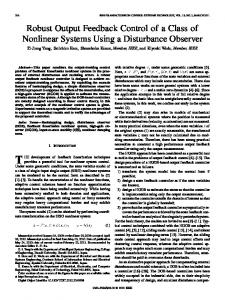
∆ϕ d x t us2 1 Qξ 3¦ xξ ¦ 2 ks1ξ2 δx ¦ xξ ¦ ξ δξξ2 ¤ ξ2 ¬λ min 1 ϕ˜ d t d x t us22 2 2 λmin Q£ ξ£¥g¤ kQ Z¦ xξ ¦ kξ ε 1 1 2 2 2 in which δx ¦ xξ ¦ ξ 2 kQ ¦ xξ ¦ 2kQ δx ξ has been used. Thus noting condition i of (37), we ¤ have V˙s λV Vs ε (42) which leads to (39) and proves result A of Theorem 2. Noting condition ii of (37), B of Theorem 2 can be proved using a positive definite function Va of the form (18) and the same technique as in (19) and (20). IV. E XPERIMENT R ESULTS To illustrate the above designs, a two-axis positioning stage shown in Fig.1 is used as a case study. The two axes of the X-Y stage are mounted orthogonally on a horizontal plane with the Yaxis on top of the X-axis. A particular feature of the set-up is that the two linear motors are of different types: the X-axis is driven by an Anorad LCK-S-1 linear motor (iron core) and the Y-axis is driven by an Anorad LEM-S-3-S linear motor (epoxy core). The position of the stage is measured by means of two optical linear encoders with the resolution of 1µm after quadrature. Experiment results are obtained for the Y-axis whose simplified dynamics is given by
(37)
530
x˙1 x2 M x˙2 u Bx2 Ff n x2 y x1
d x t !
(43)
The design parameters of the adaptive robust repetitive controller are chosen as: l1 ® 200 ° k ® 20 ° ke ® 20 ° ka ® 20 ° ε ® 1 ° Γ ® 50 ° ϕmax ® 2 ° ϕmin ® µ 2 ° dmax ® 1 ° ϕˆ d ² 0 ³�® 0 ¹
(50)
For comparison purpose, a discrete-time repetitive controller [3], [16], [17] which was proposed to solve a set-point regulation problem is also implemented: Gr ² q º
Fig. 1. X-Y stage
where x ®m¯ x1 ° x2 ± T represents the position and velocity of the inertia load, M is the unknown inertia of the payload plus the coil assembly, B is the unknown damping constant, u is the control voltage, Ff n is the unknown nonlinear friction force, and d ² x ° t ³ represents the lumped disturbance consisting of model uncertainties and external disturbances. The controller design proposed in Section III can be generalized to solve the tracking control problem of the linear motor. For simplicity, the dynamic compensator (25) is ignored, i.e., Cc ® 0. Thus the switching-surface-like tracking error is given by ξ ® e˙1 ´ l1 e1
®
x2 µ x2eq °
x2eq
® ∆ y˙d µ
l1 e1 °
(44)
where e1 ® y µ yd . Differentiating (44) and substituting the expression given by (43), one obtains M ξ˙ ® u ´ ϕ ´ d °
(45)
where ϕ ® µ M x˙2eq µ Bx2 µ Ff n ² x2 ³ . Adding and subtracting a repeatable term ϕd ² t ³.® µ M y¨d µ By˙d µ Ff n ² y˙d ³ on the righthand side of (45) yields ∆
M ξ˙ ® u ´ ϕd ² t ³
´
∆ϕ ´ d °
(46)
where ∆ϕ ® ϕ µ ϕd . As shown in [4], ∆ϕ can be quantified as
¶
∆ϕ
¶¥·
¶ ¶
γ1 e1
´
¶ ¶
γ2 e21 ´ γ3 ξ
´
¶ ¶¬¶ ¶
γ4 ξ e1
°
µ
kξ µ ke e1 µ ka e21 ξ ° us2
® µ
1 2 4ε h ξ
°
(48)
where h is defined in Remark 1, and the controller parameters k, ke and ka are positive scalars satisfying the following conditions: ka
¸
γ2 ´ γ4 ° ke l1
¸
1 1 γ1 ´ γ2 ° k 2 4
¸
1 1 γ1 ´ γ3 ´ γ4 ¹ 2 4
The associated learning algorithm is given in (35).
º N ² 1 µ 1 ¹ 96q º 1 ´ 0 ¹ 9608q º 2³ Q ² q º 1 ³ ³�® ² 0 q0151q º 1 µ 0 ¹ 01431q º 2³!² 1 µ Q ² q º 1 ³ q º N ³ ° ¹
(51) where q is the one step delay shift operator, N ® 100, and the Q filter is chosen as Q ² q º 1 ³�®»² q ´ 2 ´ q º 1 ³�¼ 4. Both controllers are implemented using a dSPACE DS1103 controller board and the sampling rate is fs ® 10KHz. First we consider a set-point regulation problem when the linear motor is disturbed by a sinusoidal disturbance d ² t ³½® 0 ¹ 2 sin ² 200πt ³!² V ³ . The performance of the discrete-time repetitive controller and the adaptive robust repetitive controller is shown in Fig. 2 and Fig. 3, respectively. It can be seen that both controllers can eliminate the effect of the disturbance after 5 ¾ 6 periods. However, the proposed controller has a better transient performance. The motor is then controller by the adaptive robust repetitive controller to track a desired trajectory yd ® 0 ¹ 05 ¯ 1 µ cos ² 2πt ³ ± ² m ³ . The tracking error is shown in Fig. 4. It can be seen that the transient tracking error is relative large. However, it becomes smaller and smaller after several runs. This result shows that the control algorithm ensures the convergence of the output tracking error. To test the performance robustness of the algorithms to parameter variations, the motor is run with a 9.1kg payload mounted on it. The tracking error is given in Fig. 5. It shows that controller achieves good tracking performance in spite of the change of inertia load. Finally, to test the performance robustness of the controller to disturbance, a step disturbance (a simulated 0.5V electrical signal) is added at t=4s. The tracking error is very large when the disturbance occurs (Fig. 6). But the learning algorithm captures its effect after several runs and compensates it quickly. This result illustrates the performance robustness of proposed scheme. V. C ONCLUSION
(47)
where γ1 ° γ2 ° γ3 , and γ4 are positive bounding constants that depend on the desired trajectory and the physical properties of the linear motor. Similar to [15], the adaptive robust repetitive control law is given by: u ® ua ´ us1 ´ us2 ° ua ® µ ϕˆ d ² t ³ ° us1 ®
1
(49)
In this paper, a performance oriented adaptive robust repetitive control law has been constructed for a class of n-th order uncertain nonlinear systems in a normal form. Like other existing repetitive control schemes, the proposed approach exploits the property of repetitive tasks. As a result, in the absence of non-periodic exogenous disturbances, the effect of unknown dynamic model is eliminated. In addition, by utilizing certain prior information about the system such as the bounds of the periodic uncertainties, the proposed scheme uses a projection mapping for a stable learning process – a robust performance that the existing repetitive controllers cannot achieve. Certain robust feedback is constructed to attenuate the effect of both model approximation errors and non-periodic uncertain nonlinearities for a guaranteed robust performance in general. By doing so, the presented design enjoys the benefits of both repetitive control and fast robust feedback while naturally overcoming their
531
practical limitations. The proposed scheme is implemented on a linear motor drive system, and experiment results are presented to illustrate its effectiveness.
15
[5] [6] [7] [8] [9] [10] [11] [12]
[13] [14]
[15] [16]
[17]
−5
0
0.01
0.02
0.03
0.04
0.05
0.06
0.07
0.08
0.09
0.1
Time (sec)
Fig. 3. Adaptive robust repetitive controller: set-point regulation
40
30
20
Tracking Error (µ m)
[4]
10
0
−10
−20
−30
−40
0
0.5
1
1.5
2
2.5
3
3.5
4
4.5
5
Time (sec)
Fig. 4. Tracking error for a sinusoidal trajectory without load
40
30
20
Tracking Error (µ m)
[3]
5
0
10
0
−10
−20
−30
−40
0
0.5
1
1.5
2
2.5
3
3.5
4
4.5
5
Time (sec)
Fig. 5. Tracking error for a sinusoidal trajectory with load
15 50
40
10
30
Tracking Error (µ m)
[2]
M. Krstic, I. Kanellakopoulos, and P. V. Kokotovic, Nonlinear and adaptive control design. New York: Wiley, 1995. S. Hara, Y. Yamamoto, T. Omata, and M. Nakano, “Repetitive control system: a new type servo system for periodic exogenous signals,” IEEE Trans. on Automatica Control, vol. 33, pp. 659–668, 1988. M. Tomizuka, T. C. Tsao, and K. K. Chew, “Analysis and synthesis of discrete time repetitive controllers,” ASME J. of Dynamic Systems, Measurement and Control, vol. 111, pp. 353–358, 1989. N. Sadegh, R. Horowitz, W. W. Kao, and M. Tomizuka, “A unified approach to the design of adaptive and repetitive controllers for robotic manipulators,” ASME J. of Dynamic Systems, Measurement, and Control, vol. 112, no. 4, pp. 618–629, 1990. R. Horowitz, “Learning control of robot manipulators,” ASME J. of Dynamic Systems, Measurement, and Control, vol. 115, pp. 402–411, 1993. S. Arimoto, T. Kawamura, and F. Miyazaki, “Bettering operation of robots by learing,” Journal of Robotic Systems, vol. 1, no. 2, pp. 123–140, 1984. P. Bondi, G. Casalino, and L. Gambardella, “On the iterative learning control theory for robotic manipulators,” IEEE Journal of Robotics and Automation, vol. 4, pp. 14–22, 1988. K. L. Moore, M. Dahleh, and S. P. Bhattacharyya, “Iterative learning control: a survey and new results,” Journal of Robotic Systems, vol. 9, pp. 563–594, 1992. J. X. Xu, B. Viswanathan, and Z. Qu, “Robust learning control for robotic manipulators with an extension to a class of non-linear systems,” International Journal of Control, vol. 73, no. 10, pp. 858–870, 2000. J. J. E. Slotine and W. Li, Applied nonlinear control. Englewood Cliffs, New Jersey: Prentice Hall, 1991. B. Yao, “High performance adaptive robust control of nonlinear systems: a general framework and new schemes,” in Proc. of IEEE Conference on Decision and Control, pp. 2489–2494, 1997. B. Yao and M. Tomizuka, “Smooth robust adaptive sliding mode control of robot manipulators with guaranteed transient performance,” Trans. of ASME, Journal of Dynamic Systems, Measurement and Control, vol. 118, no. 4, pp. 764–775, 1996. Part of the paper also appeared in the Proc. of 1994 American Control Conference. S. Sastry and M. Bodson, Adaptive Control: Stability, Convergence and Robustness. Englewood Cliffs, NJ 07632, USA: Prentice Hall, Inc., 1989. B. Yao and M. Tomizuka, “Adaptive robust control of SISO nonlinear systems in a semi-strict feedback form,” Automatica, vol. 33, no. 5, pp. 893– 900, 1997. (Part of the paper appeared in Proc. of 1995 American Control Conference, pp2500-2505). L. Xu and B. Yao, “Coordinated adaptive robust contour tracking of linearmotor-driven tables in task space,” IEEE Conf. on Decision and Control, pp. 2430–2435, 2000. T. C. Tsao and M. Tomizuka, “Robust adaptive and repetitive digital control and application to hydraulic servo for noncircular machining,” ASME J. Dynamic Systems, Measurement, and Control, vol. 116, pp. 24–32, 1994. M. Tomizuka, “On the design of digital tracking controllers,” ASME J. Dynamic Systems, Measurement and Control (50th Anniversary Issue), vol. 115, no. 2(B), pp. 412–418, 1993.
Position (µ m)
[1]
Position (µ m)
10
R EFERENCES
5
20
10
0
−10
0 −20
−30 −5
0
0.01
0.02
0.03
0.04
0.05
0.06
0.07
0.08
0.09
0.1
−40
Time (sec)
0
1
2
3
4
5
6
7
8
Time (sec)
Fig. 2. Discrete-time repetitive controller: set-point regulation
Fig. 6. Tracking error for a sinusoidal trajectory with disturbance
532