Adaptive Routing Algorithm for Lambda Switching Networks Stelios Sartzetakis Institute of Computer Science - FORTH and Computer Science Dept. - University of Crete Heraklion - CRETE, GREECE GR-711 10 e-mail:
[email protected] Chrysostomos I. Tziouvaras Institute of Computer Science - FORTH and Computer Science Dept. - University of Crete Heraklion - CRETE, GREECE GR-711 10 e-mail:
[email protected],
[email protected] Leonidas Georgiadis Aristotle University of Thessaloniki Dept. of Electrical and Computer Engineering P.O. Box 435 Thessaloniki 54006, GREECE e-mail:
[email protected]
Abstract Current developments in optical components’ technologies enable wavelengths to be very narrowly spaced, transforming the optical fiber into a multi-terabit capacity medium. A new generation of “all-Optical” CrossConnects started to appear in the market leading to a number of advantages such as increased switching capacity, decreased overall network costs, scalability and transparency resulting in the capability to support any protocol. An additional advantage is the ability to configure the switching fabric and the wavelength converters in real time. For the control of Optical Cross-Connects, the MPLambdaS approach was proposed by IETF, according to which the MPLS traffic engineering control plane is used in Optical Cross Connects. New corporate services appear such as storage area networks, optical virtual private networks, while end-user broadband services like video on demand and person-to-person applications pose a huge demand to today’s providers. In this new environment the issue of resource allocation in mesh topology networks using Dense Wavelength Division Multiplexing (DWDM) is very important. In this paper an adaptive routing algorithm based on lexicographic optimization is proposed and it is examined through simulation. The experimental results show that the algorithm outperforms in terms of overall network throughput by more than 30% two well-known algorithms: shortest path and fixed paths least congested routing. For large core networks this improvement corresponds to an increase in the order of Tbps. In this paper an attempt is also made to propose a framework for the application of lexicographic optimization in large operator’s networks supporting these new services that have a dynamic behavior and the demand cannot be predicted beforehand in an accurate way. Keywords: optical networks, WDM networks, lambda switching, resource allocation, routing.
1
I. Introduction Recently, several major improvements have occurred to optical components’ technologies, which make optical networks a very attractive solution for providers. More specifically, wavelengths can now be very narrowly spaced and there are commercial products that can multiplex several hundreds of wavelengths within a single fiber. In addition, the development of “all-Optical” Cross-Connects, which switch wavelengths without transforming light to electricity, is now feasible. This improvement decreases the overall cost of the network, increases network’s capability for upgrade and makes the network transparent, hence capable of supporting every protocol/service. Furthermore reconfigurable Optical Cross-Connects are now available, that is the switching fabric and the wavelength converters can be configured in real time. For the control of Optical Cross-Connects (OXC), the MPLambdaS [1] approach was proposed by IETF, according to which the MPLS traffic engineering control plane is used in Optical Cross Connects. This approach transforms optical networks to real switched networks, from a protocol perspective, offering the flexibility and the generic capabilities that MPLS provides. New corporate services appear such as storage area networks, optical virtual private networks, while end-user broadband services pose a huge demand to today’s providers. Nowadays customers ask for network services that deliver huge bandwidth when and where they mostly need it. With increasing Internet traffic and LAN speeds, with the need to interconnect geographically separated LANs, and with the appearance of Applications Service Providers traffic growth will continue to explode. Only with the use of “all-optical” OXCs and network architecture enhancements the required capacities and flexibility could be achieved. These new optical networks are usually referred to as third generation DWDM networks. Taking into consideration the above stated technology advances and the new services environment, the problem of resource allocation in large operators’ networks was studied and the application of lexicographic optimization was examined. In the following the terms routing and resource allocation will be used interchangeably.
Evolution of architectures for Optical Cross-Connects In this section the evolution of Optical Cross-Connects’ architectures is presented [2]. The OXCs used today, called opaque OXCs, use electrical switching fabrics and static wavelength conversion. The basic architecture of these OXCs is outlined in Figure 1. The optical signal carried in each wavelength is passed to an O-E-O transponder, which converts it to the region of 1310nm. This optical signal is then converted to electrical and de-multiplexed into STS-1 signals. These signals are cross connected using an n x STS-1 matrix and then are multiplexed in order to
2
form a higher SONET rate. Then this signal is transformed to optical in the region of 1310nm and finally converted to the appropriate output wavelength with the use of an O-E-O transponder that does static wavelength conversion. One of the disadvantages of this architecture is that it uses electric switching fabric, which does not scale well. In addition it is very expensive because it involves a large number of O-E-O conversions, which are six per wavelength, and one transponder per wavelength. Furthermore this architecture is based on SONET and the fact that the optical signal is de-multiplexed to STS-1 rates implies that this architecture leads to bottlenecks, as the number of wavelengths and the transport capacity of each wavelength increase. For instance assume an OXC that terminates 25 fibers, where each fiber can multiplex 160 wavelengths. This implies that the OXC must be able to switch 4000 wavelength connections. It is obvious that for such figures, which are expected to be commonplace soon, this architecture is not appropriate.
1310 nm
Fiber1
λ1
OEO transponder Static wavelength conversion
OE transponder
Electrical switching fabric
Static wavelength conversion EO transponder
OEO transponder
λ2
Fiber2
1310 nm
Optical (O-E-O) Cross Connect
Figure 1: Existing Optical Cross-Connects An evolution to this architecture is the one that uses optical switching fabric, developed using technologies such as Micro Electro Mechanical Systems (MEMS) and liquid crystals. The optical switching fabrics are expected to scale in a more cost-effective way than the electrical switching fabrics and they can scale to several thousands ports. However this architecture does not provide transparency because it involves the use of O-E-O transponders per wavelength as shown in Figure 2. This means that a great number of transponders are required due to the increasing number of wavelengths that can be multiplexed within a fiber. In addition this architecture uses static wavelength conversion, which implies that in order to resolve wavelength contention the optical signal must pass through a number of O-E-O transponders. Hence despite the fact that this architecture manages to reduce the number of O-E-O conversions per wavelength in comparison with the previous, it remains very expensive. Furthermore this architecture is also bit-rate dependent, which means that upgrades in wavelengths’ transport capacity involve serious hardware changes.
3
Fiber1
λ1
1310 nm OEO transponder Static wavelength conversion
Static wavelength conversion
Optical switching fabric
OEO transponder
λ2
Fiber2
1310 nm
Optical Cross Connect
Figure 2: Optical Cross-Connect with optical switching fabric A variant of the previous architecture uses transponders only to the OXCs that are at the edge of the network. Hence the OXCs at the core of the network are transparent, but they cannot divide the particular wavelengths and they switch them according to the band that they belong. The disadvantage of this architecture is that it can lead to fiber under-utilization. Enabled by a new generation of optical components such as tunable lasers and filters the third generation OXC is the “All-Optical” Cross-Connect. This architecture makes use of optical switching fabrics and transparent wavelength converters, which eliminate the need for O-E-O transponders. One version of this architecture is shown in Figure 3. According to this, the wavelength that arrives into an OXC is converted to a particular wavelength with the use of a tunable converter without being transformed to electricity. It is then passed to the optical switching fabric, which routes the optical signal to the appropriate output fiber.
Fiber1
λ1
Tunable lambda conversion
λ2
Optical switching fabric
λ2
Fiber2
Figure 3: Third generation “All-Optical” Cross-Connect This architecture has obviously some important advantages in comparison to the previously mentioned. First of all this architecture is totally transparent, that is the optical signal does not need to be transformed to electricity at all; this implies that this architecture can support any protocol and any data rate. Hence, possible upgrades in wavelengths transport capacity can be accommodated at no extra cost. Furthermore, it decreases the cost because it involves the use of fewer devices than the other architectures. In addition, transparent wavelength conversion eliminates constraints on conversions. In this way the real switching capacity of the OXC is increased, leading to cost reduction. Products that are based on this architecture are expected to be available very soon.
4
Control of Optical Cross-Connects The MPLambdaS approach For the control of all kinds of OXCs, the Multi-Protocol Lambda Switching (MPLambdaS [1]) approach was proposed by IETF. According to this approach, the MPLS traffic engineering control plane is used as the control plane of the OXCs. This concept originated from the observation that an MPLS capable IP router, which is called Label Switching Router (LSR), and an OXC have many similar functional characteristics. First of all, they both decouple the control plane from the data plane. From a data plane perspective, an LSR switches packets according to the label that they carry. An OXC uses a switching matrix to connect an optical signal from an input fiber to an output fiber. From a control plane perspective, an LSR bases its functionality on a table that maintains relations between incoming label/port and outgoing label/port. An OXC bases its functionality on a switching matrix that maintains relations between incoming wavelength/fiber and outgoing wavelength/fiber. It must be pointed that in the case of the OXC, the table that maintains the relations is not a software entity but it is implemented in a more straightforward way, e.g. by appropriately configuring the micro-mirrors of the optical switching fabric. There are several constraints in re-using the MPLS traffic engineering control plane. These constraints arise from the fact that LSRs and OXCs use different data technologies. More specifically, LSRs manipulate packets that bear an explicit label and OXCs manipulate wavelengths that bear the label implicitly; the wavelength itself is the label. However the use of different data technologies is not a restrictive constraint; the MPLS control plane has been already used in ATM and Frame Relay networks [3], [4]. The fact that OXCs manipulate wavelengths is because optical packet processing is infeasible with existing optical technology. There are predictions that optical packet processing will be feasible in about ten years time [5]. Hence, due to technology constraints, OXCs do not support label merging and stacking can have a finite small depth. In addition, the granularity of the wavelengths can be discrete (OC-48, OC-192 or OC-768) in comparison with the granularity of a CR-LSP, which is restricted by the maximum bandwidth that can be allocated. In order to transfer the MPLS traffic engineering control plane to OXCs certain extensions to the signaling protocols of MPLS (CR-LDP [6], RSVP [7]) as well as to the standard IP routing protocols (OSPF [8], IS-IS [9]) were proposed. These extensions take into consideration the inherent peculiarities of the optical network. The MPLambdaS approach seems to have a strong industry momentum. There are already many manufacturers that have announced the development of OXCs that use the MPLS traffic engineering control plane.
5
The main advantages of the MPLambdaS approach involve that it offers a framework for real-time optical path establishment. In addition it uses already existing and deployed protocols while it simplifies network management because this can be performed in a unified way in both the data and the optical domain. Furthermore, it offers a functionality framework that can accommodate future expectations concerning the way networks will work and the way services will be provided to clients.
Architectural models Existing optical networks are modeled as shown in Figure 4 and Figure 5; there’s a core optical network that consists of OXCs and there are several client networks, consisting of LSRs, which are attached to it. When deploying MPLambdaS in optical networks, the interaction between the control plane of the OXCs and the LSRs is an issue. In other words what the interaction between the optical network and the client networks has to be specified. Two main architectural models have been proposed [10] •
Overlay model: according to this, different instances of the control plane are used for the OXCs and the LSRs. Each instance of the control plane operates independent of the other and there’s minimum interaction between the two. Signaling and routing are performed independently in the optical and the client networks. The interaction between the client networks and the optical network is performed through signaling at the User-toNetwork Interface (UNI) in a client-server fashion. The signaling protocols of MPLS have been appropriately extended in order to support this functionality [11], [12]. Hence client networks have no access to the internals of the optical networks and they perceive the optical network as the set of established optical paths that they use (see Figure 4).
•
Peer model: according to this, a single instance of the control plane is used for both the OXCs and the LSRs. Signaling and routing is performed in a “uniform” way, as if the optical network and the client networks belonged to the same autonomous system. Hence client networks can have access to the internals of the optical network and they can ask for the establishment of an optical path by specifying the OXCs that will traverse (see Figure 5).
Examining these architectural models, it can be argued that they correspond to different operational environments; if the optical network and the client networks belong to different business entities who do not provide access to each others’ network internal information, then the overlay model must be utilized. The overlay model is simpler and allows separate development of the optical network and the client networks. On the other hand, the peer model
6
involves the exchange of large amount of control information, which in many cases is not of much use, but it allows the development of unified traffic engineering schemes that optimize the utilization of the optical network and the client networks in dynamic data environments. Other than these extreme architectural models, hybrid models can also be applied. For instance, in the peer model routing hierarchies can be employed so as to limit the control information that is exchanged and hence to improve scalability.
Optical Network UNI
UNI
Figure 4: The overlay model
Optical Network
Figure 5: The peer model
A brief review of routing in optical mesh networks In the following a brief review of routing in optical mesh networks is made. The issue of wavelength assignment is not considered here because based on developments in the market it is assumed that in the near future OXCs will be equipped with wavelength conversion capabilities. In this way routing constraints are eliminated (wavelength continuity constraint) and the optical network can be utilized in a more efficient way.
7
Basic routing approaches The basic routing approaches for optical mesh networks that can be found in the literature are [14]: •
Fixed routing: in order to satisfy connection requests it always makes use of a fixed route for a particular source-destination pair. An example is fixed shortest path routing; according to this the shortest path for each source-destination pair is calculated and any connection request between a pair of nodes is served using the path that was previously calculated.
•
Fixed alternate routing: it is different than fixed routing in that it calculates a set of paths for each sourcedestination pair. Among the paths that belong to this set there’s an ordering which defines how desirable is the use of the particular path. An example is that the set of paths for source-destination pair consists of the shortest path and the second shortest path, in this ordering. When a connection request for a particular source-destination pair arrives, the source node tries to serve it using the previously calculated shortest path. If this path is not available, then the source node tries to serve the request using the previously calculated second shortest path. If this isn’t available too, then the request is blocked.
•
Adaptive routing: it chooses the paths in a dynamic way, taking into consideration the current network state. An example is the fixed paths least congested routing algorithm [19]. This algorithm takes into consideration the current network state, because the number of currently allocated wavelengths on a link defines its cost. When a connection request for a particular source-destination pair arrives, then the source node chooses the path with the minimum sum of costs.
Fixed routing is the simplest approach and adaptive routing the more complex. However adaptive routing achieves the best performance in terms of blocking. Fixed alternate routing stays in the middle offering a trade-off between complexity and performance. Common methodologies for routing in optical mesh networks The selection of the appropriate routing methodology in DWDM networks is dictated by the assumptions concerning the way the requests arrive. There are two categories concerning traffic assumptions [15]: static and dynamic. In the static case the demand for each source-destination pair is known beforehand. Usually the objective here is to minimize the number of wavelengths that must be used in order to satisfy the demand or to maximize the number of the optical paths for a given fixed set of wavelengths. In the dynamic case optical paths are setup and released dynamically, hence there’s no prior knowledge about the actual demand. The objective in this case is to minimize blocking probability or to maximize the number of established optical paths at any time.
8
Algorithms that assume a static traffic model, usually do not take into account all possible paths for a sourcedestination pair because the number of these paths increases exponentially with the number of network nodes and links. Usually a set of available paths is calculated based on the shortest path algorithm. In the case where there are more than one available path to choose, two classes of algorithms are generally employed: sequential and combinatorial algorithms. Sequential algorithms examine each source-destination pair and choose the appropriate path or paths according to a routing criterion and then visit another source-destination pair, without changing previous allocations. The sequence that the source-destination pairs are visited affects the total number of established optical paths and this dependency is not an obvious one. Combinatorial algorithms calculate optical paths in a global way. These algorithms can be categorized as optimal and heuristic. Optimal algorithms optimize a particular objective and can be formulated as a mixed-integer linear programming problem. The disadvantage of this kind of algorithms is that they are NP-complete. Heuristic algorithms try to converge to the optimal solution but without caring for 100% accuracy. Obviously, they give worse results than optimization algorithms but are much simpler. The problem of routing assuming a dynamic traffic model is much more difficult than the problem of routing assuming a static traffic model. This is because it bears the additional constraint that its solutions must be simple and fast so as to be able to handle the arriving requests quickly. For this reason heuristics are generally employed.
Proposed routing algorithm In this paper an algorithm for routing in DWDM network is examined. This algorithm calculates optical paths in such a way so as the vector of link costs is lexicographically optimal [16], where the cost of a link is defined as the number of previously allocated wavelengths. Hence, it is a “pure” load balancing algorithm and as such it ensures that •
Network availability for new connections is evenly distributed over the whole network. Hence the network can accept unpredictable traffic reservation requests.
•
There’s diversity between the chosen optical paths, which increases network’s robustness in case of component failures.
According to the classification shown in the previous section this algorithm is adaptive, because the costs of the links are continuously updated so as to indicate the current level of load. Concerning the traffic assumptions, a static traffic model was assumed.
9
The proposed algorithm finds the lexicographically optimal solution for a source and a set of destinations. For linear link costs, the algorithm’s complexity is O(N5), where N is the number of the nodes of the network [16]. In this paper a heuristic is proposed in order to converge to the globally lexicographically optimal allocation. Such an allocation guarantees that the maximum number of connections is achieved in comparison with every other allocation algorithm, which leads to the greatest profit for the owner of the optical network. Hence, the main advantages of the algorithm are that it has polynomial complexity and by using a simple heuristic a step towards the globally lexicographically optimal allocation is performed. In addition, the use of lexicographic optimization is examined in a highly dynamic data environment, as the one that is predicted to prevail in the near future, in which the table of demand simply provides an indication of the actual demand that will be expressed. In order to accommodate for this, a management scheme is proposed which performs, locally or globally, corrective actions when the traffic diverges significantly from the predicted load, in order to guarantee network’s efficient operation.
II. Routing in optical mesh networks using lexicographic optimization A short introduction to the issues concerning lexicographic optimization and a simple example is given. The algorithm that calculates the lexicographically optimal paths was introduced in [16] where it is thoroughly described. Then alternative ways to deploy it in optical mesh networks are examined. Early results of this work were presented in [17].
Lexicographically optimal allocation The formal definition of lexicographic ordering follows: Given an n-dimensional real vector x define by
φ (x)
the n-dimensional vector whose coordinates are those of x
arranged in non-increasing order, i.e.
φ ( x) = (φ1 ( x), φ2 ( x),..., φn ( x)) = ( xi , xi ,..., xi ) 1
where
2
n
xi1 ≥ xi2 ≥ ...≥ xin
Then, vector x is called lexicographically smaller than or equal to vector y , if either exists a number l , 1 ≤ l ≤ n , such that
φ ( x) = φ ( y ) , or there
φ i ( x) = φ i ( y) , for 1 ≤ i ≤ l − 1 and φ l ( x) p φ l ( y ) .
The optical paths are calculated in such a way so as the vector of the number of allocated wavelengths in the links of the network is lexicographically minimum.
10
The lexicographically optimal allocation leads to a unique allocation that belongs to the family of solutions of the well-known min-max algorithm. The min-max algorithm provides a means for allocating bandwidth in the maximally loaded links of the network without caring about the less loaded links of the network, so it provides a family of solutions. The next figures clarify the difference between the min-max allocation and the lexicographically optimal allocation. Assume that four wavelength paths must be chosen from source node A to destination node H. Notice that the minmax allocation (Figure 6) selected two routes and totally six links have two allocated wavelengths. In the lexicographically optimal allocation (Figure 7) four routes are chosen and only two links have two allocated wavelengths. Intuitively the lexicographically optimal allocation leads to a more balanced network.
B
2
2
D 2
A C
H
2
2
F
2
E
G
Figure 6: Min-max allocation B
1
1
D 2
1
A
1
C 1
2
H
F
1
E
1 1
G
Figure 7: Lexicographically optimal allocation
Deployment scenarios In deploying lexicographic optimization for calculating optical paths it was assumed that there’s a table of demand that defines the needs for optical paths for every source-destination pair. A realistic assumption given that providers usually build such tables using existing contracts with clients and predictions (long term network planning phase).
11
Two ways were considered for deploying lexicographic optimization; serial deployment and iterative deployment. In serial deployment, for every source node the optical paths are calculated to all other destinations in one step, until the paths for all sources are calculated. The order in which source nodes are chosen affects the final results, so in the experiments that were conducted a random order of source nodes was chosen. In iterative deployment the paths are calculated in a serial way, as before, and then they are re-calculated until there’s a convergence to a solution. The heuristic is shown in Table 1.
Given a topology and a demand table, 1.Initially assume that no reservations exist in the network 2.For i=1 to k do //where k is the number of source nodes 3.Find the lexicographically optimal allocation from source node i to all destinations, according to the demand table, keeping the allocations of the other source nodes fixed 4.End do 5.If the new allocations on the links and the allocations before the FOR loop differ by more than a small value ε then go to step 2; Else STOP.
Table 1:The heuristic for iterative deployment In essence, this heuristic is an effort to converge to the globally lexicographically optimal allocation. It cannot be argued that the heuristic converges to this allocation, because this is something that must be formally proven. However, as will be shown in the next section, experimental results show that this heuristic provides better results compared with the serial deployment. It can be easily proven that the globally lexicographically optimal allocation can accommodate more optical paths than any other resource allocation algorithm. Hence, there’s strong motivation in pursuing the globally lexicographically optimal allocation.
12
III. Experimental results Experimental environment In order to conduct experiments a simulator was developed in C++ using the LEDA package [18], which is one of the most reliable packages for developing graph algorithms. For the experiments a real world topology was used, the North America network of Global Crossing. The reason for using an existing topology instead of using a random one is that fibers are already installed and it is rather unrealistic to assume very different physical topologies for the immediate future.
Figure 8: The experimental topology For every link of the network it was assumed that there’s a pair of fibers of opposite direction and that every fiber multiplexes 128 wavelengths. A table of demand was created in such a way so as to create congestion. The reason for this is that in congestion conditions the algorithm’s performance can be evaluated more effectively.
Experimental Results The algorithm that calculates the lexicographically optimal allocation was compared with the following algorithms •
Shortest path: a non-adaptive algorithm in which every fiber has equal cost. It chooses the path with the minimum sum of costs as long as this path is not blocked.
•
Fixed paths least congested routing [19]: an adaptive algorithm in which every fiber has cost equal to the number of wavelengths which where previously allocated. It chooses the path with the minimum sum of costs as long as this path is not blocked. In [19] it is proposed to take into consideration only a set of predetermined paths. In the experiments that were conducted all the available paths were taken into consideration, hence this version of the algorithm will have better performance than the one proposed in [19].
13
The metric that was used in order to evaluate the algorithms’ performance was the percentage of the established optical paths with reference to the total number of the requested optical paths by the table of demand. A great number of experiments were conducted for the above topology by using different order of selecting source nodes. The results that are shown below are the average values of the experiments’ output. The experimental results for the serial deployment are shown in Figure 9. As the results indicate the serial deployment of the lexicographic optimization strongly outperforms both shortest path and fixed paths least congested routing. By doing the appropriate reductions, the serial deployment of lexicographic optimization outperforms shortest path by 37.5% and fixed paths least congested routing by 34.6%. Considering that every optical path has capacity in the order of Gbps, the results indicate that for large topologies, as the one that was considered in the experiments, the improvement in the total network’s throughput can be in the order of Tbps. Hence, it corresponds to a great profit increase for the provider. 100,0% 87,9%
90,0% 80,0% 70,0%
63,9%
65,3%
Shortest Path
Fixed paths least congested routing
60,0% 50,0% 40,0% 30,0% 20,0% 10,0% 0,0% Serial deployment of lexicographic optimization
Figure 9: Experimental results for serial deployment of lexicographic optimization The experimental results for the iterative deployment of the lexicographic optimization are shown in Figure 10. 90,2%
90,5% 90,0% 89,5% 89,0% 88,5% 88,0%
87,9%
87,5% 87,0% 86,5% Serial deployment of lexicographic optimization
Iterative deployment of lexicographic optimization
Figure 10: Experimental results for iterative deployment of lexicographic optimization The results indicate that the iterative deployment of the lexicographic optimization slightly outperforms the serial deployment by about 2.6%.
14
The fact that the improvement is small cannot be an argument against the use of the iterative deployment of the lexicographic optimization. The reason for this is that other topologies were found where the improvement was much greater. More specifically consider the topology shown in Figure 11 and the table of demand that is shown in Table 2. C
F
A
I D
G
B
G
E
H
Figure 11: Example topology where iterative deployment of lexicographic optimization performs much better than serial deployment Source A B
Destination I G
# optical paths 90 90
Table 2: The demand table
Assuming that every fiber can multiplex 60 wavelengths, serial deployment of lexicographic optimization manages to establish 90+75=165 optical paths. On the other hand the iterative deployment of lexicographic optimization manages to establish all the requested optical paths. By doing the appropriate reductions, this corresponds to about 9% improvement. Hence the use of the iterative deployment is justified. Notice also, that the only overhead that the iterative deployment adds in comparison to the serial deployment, is more processing time, which is the time of the serial deployment multiplied by the number of FOR loops. As will be explained in the next section the use of the lexicographic optimization will be off-line, so time is not an important consideration. In addition, the experiments indicate that the heuristic for the iterative deployment is quite stable and converges on an average within 7 FOR loops, which is considered a small number of loops. As stated earlier this heuristic is an effort to converge to the globally lexicographically optimal allocation. In the experiments for the Global Crossing’s network one cannot prove that this was achieved. However contacting
15
experiments for smaller topologies, as the one that is shown in Figure 11 where the globally lexicographically optimal allocation was known beforehand, showed that the heuristic converged to the optimal allocation.
IV. A business model for applying lexicographic optimization in dynamic environments The network model It is evident that current static data profiles are transforming to more dynamic data paradigms. This evolution is feasible by the advances in the OXCs’ architecture and the deployment of MPLambdaS, which offer the potential for real-time optical path establishment. Hence in the near future, a client network that is attached to an optical network is not expected to make long-term contracts leasing one or more optical paths but it will dynamically purchase and release optical resources based on its current needs. Having this environment in mind, a framework is proposed for using lexicographic optimization. A network model that consists of the following two kinds of devices is assumed: 1.
Ordinary IP routers that are MPLS enabled (LSR).
2.
Generic devices (LSR/OXC) that combine the functionality of a common LSR and of an Optical Cross-Connect (OXC)1. They have both electrical ports and optical ports; hence they can aggregate smaller granularity “electric” traffic (CR-LSPs) into wavelengths. It is assumed that these devices function according to the MPLambdaS approach.
The network model is shown in Figure 12.
Client Network
Optical Network Client Network
Client Network
Client Network
Client Network
Figure 12: The network model 1
The reason for not using pure OXCs is that they do not have “electronic” aggregation capabilities so they cannot interface with customers. Hence, there’s no economic incentive for their use.
16
The client networks that connect to the optical network can be ISPs or enterprise networks. It is assumed that the client networks are MPLS capable so they consist of LSRs. The optical network consists of the generic devices (LSR/OXC) described above. To every device of the optical network one or more client networks are attached. The functionality framework that will be presented applies for large operators’ networks; in this environment the overlay model seems more appropriate, because operators usually do not provide information concerning their network to clients. Hence in the following, it is assumed that the client networks interact with the optical network according to the overlay interconnection model. Client networks generate requests for the establishment of CR-LSPs that traverse the optical network. These requests are translated into requests for optical path establishment. After the optical path has been established subsequent CR-LSP requests use this optical path as a normal link (forwarding adjacencies[20]), which means that the CR-LSPs are tunneled through the optical path [13]. Hence in the network model it is assumed that every optical path can be used by many client networks’ CR-LSPs. This implies that charging occurs according to the portion of the wavelength that the CR-LSP occupies. However, in the proposed model the possibility of a client network asking for a whole optical path is not excluded. The question whether an optical path will be of exclusive use for a particular client network is explicitly specified before the actual establishment of the optical path e.g. in CR-LDP is specified in the Label_Request message (Contact Id attribute of Service TLV [11]). Within the optical path ultra fast layer 1 forwarding is performed, that is every intermediate LSR/OXC makes use of the capabilities of a pure OXC that it has. Notice that within the optical path full transparency is maintained for the smaller granularity CR-LSPs. When the light reaches the last LSR/OXC of the optical path, then it is transformed to electricity, all packets are examined concerning the MPLS label that they carry and are sent to some destination accordingly.
Management of CR-LSP establishment requests In the case where optical paths are used by a number of client networks2, an important issue is when to establish a new optical path. When a new CR-LSP request arrives a policy server[11] examines the request and decides how the request can be served. Three alternatives are possible 1.
Use an existing optical path that connects the requested optical endpoints.
2.
Use more than one existing optical paths that lead to the requested optical endpoint.
3.
Establish a new optical path.
2
The case that a client network asks for a whole optical path is straightforward; the path is provided for use only to the particular client network
17
Alternative (1) is the obvious solution because it makes little use of optical resources. However there are cases where it cannot be used; such cases include existing paths do not have the requested bandwidth or the requested CRLSP characteristics (e.g. protection) are not supported by the existing optical paths. Alternative (2) has the same constraints as (1), but it carries the extra overhead that in general uses additional optical resources, in terms of total number of hops to the destination. By putting an upper limit on the number of the optical paths that can be used this overhead can be controlled. Alternative (3) entails the danger of under-utilization; the establishment of an optical path, which is in the order of Gbps, is triggered by a request for the establishment of a CR-LSP, which is in the order of Mbps. Hence if subsequent demand is not adequate there will be low utilization for the optical path, something that is not desirable for the owner of the optical network. The policy server must examine the possibility of underutilization before deciding to establish a new optical path. Elements that could be taken into consideration include the requested CR-LSP’s class, the client that produced this request and the bandwidth granularity of the request. An interesting tradeoff is between alternatives (2) and (3). One could argue that alternative (3) must be deployed when alternative (2) cannot serve the request. The disadvantage of this approach is that every CR-LSP utilizes a number of optical paths, which implies that the overall network’s throughput is far from being optimized. In general it can be argued that the most suitable approach would be to use alternative (2) when the policy server decides that the risk of under-utilization for a new optical path exceeds a certain threshold.
The business model This section describes a framework in which the proposed lexicographic optimization for large optical mesh networks, where data traffic exhibits dynamic behavior, could be beneficial. In this framework optical path establishment requests are dealt with, which implies that the actions described below happen when the policy server decides the establishment of new optical paths. The use of this algorithm is best suited for this environment since it results in evenly loaded networks of highly balanced availability. It is assumed that there’s an initial table of demand that defines the number of optical paths that must be established between every pair of nodes. This information can be derived by existing contracts with clients and the provider’s predictions. However, it is hard to assume that the table of demand could be accurate because of the high degree of uncertainty concerning the arrival for requests for optical path establishment and the time the optical paths will be active. Hence, it can be argued that the table of demand expresses only a prediction about the average needs for optical paths for every pair of nodes.
18
Given the demand table, the actual paths are calculated by a centralized entity, using the iterative deployment of the lexicographic optimization, which is more effective than the serial one, as indicated by the experimental results. The calculated paths are then “downloaded” to the source nodes using a management protocol. These paths are not established until a request for a path has arrived. The flowchart depicted in Figure 13 shows what is happening when a request for an optical path arrives.
Request for optical path between (s,d)
1.Are there any stored and unused paths between (s,d)?
YES
2.Establish the path using the stored paths
NO 3.Is the rate of "excess" paths larger than a threshold?
NO
YES
4.Are there available paths?
YES
5.Establish the path using lexiocgraphic optimization
NO
6.Perform local optimization
7.Was the request satisfied?
NO
8.Perform global optimization
Figure 13: Sequence of actions when a request for optical path establishment arrives When a request for optical path establishment arrives, the source node checks if there’s a stored path that has not been allocated yet. If there is such path then it uses it to satisfy the request. If there is no such path, then the source node checks if the rate of the paths that have been established without using the stored paths (because they were previously allocated) exceeds a threshold posed by the provider. The meaning of this check is to find whether the requests from this node have highly exceeded the prediction, as indicated by the demand table, in such a degree that puts in jeopardy the optimized usage of the network, as calculated by the iterative deployment of the lexicographic optimization. If the answer to question 3 is yes, then some action must be taken in order to ensure that network usage is optimized even in such conditions where the requests exceed the prediction. This action is performed by local optimization, according to which the allocated optical paths starting from the particular source node that were not established using the stored paths, plus the new request are re-calculated using lexicographic optimization.
19
It is clear that local optimization involves rerouting of existing optical paths. This does not imply service disruption because the mechanism for rerouting CR-LSPs [21] defines that the new CR-LSP is constructed prior to the deletion of the old CR-LSP. If the answer to question 3 is no, then the source node checks whether there are available resources that can form a path to the particular destination. This check is straightforward because assuming that every LSR/OXC device uses the MPLS traffic engineering control plane, the routing protocols have been appropriately extended and every node has knowledge about the available resources of the network. If there are available resources then the node calculates a new path using lexicographic optimization. If there are not available resources then local optimization is performed. Notice that local optimization has much more possibilities to be successful when is activated by question 3 rather than question 4. This is because when there are no available resources the network faces more severe congestion with regards to the requests entering from the particular node. If local optimization is not successful, that is there were not available resources to accommodate the rerouted optical paths plus the new request, then there’s severe network congestion and the problem must be globally solved. This is performed by global optimization. It is assumed that during normal network operation the table of demand is continuously updated, taking into consideration current conditions. Hence, when global optimization is activated a new table of demand is ready for use and all optical paths are re-calculated using the iterative deployment of lexicographic optimization. In other words, global optimization is used as a control mechanism that sets the network in an efficient operation for a particular window of time. The action global optimization corresponds to time in the order of a month and obviously every provider wants to be triggered as rarely as possible. The actual time between two successive global optimizations depends on the accuracy of the demand table. The action local optimization corresponds to a different time scale, in the order of a day. The flowchart that was presented in Figure 13 is a framework for the network’s operation and it is open to modifications according to the provider’s goals. For instance, one could argue that it is not necessary to activate local optimization whenever there are not available paths (question 4) because of the dynamic character of the optical paths’ allocation; soon after the request arrives, an optical path may be released and the request can be satisfied without performing local optimization. Hence, an alternative criterion for activating local optimization could take into consideration the rate of rejected requests within a window of time. In addition, global optimization may not necessarily be activated whenever local optimization fails, because global optimization affects whole
20
network’s operation. Hence an alternative criterion for global optimization’s activation could take into consideration failures of local optimizations of different nodes within a window of time.
Fault management Up to now, there’s no mention made for network’s protection and restoration. However it has already been mentioned that lexicographic optimization balances the load as even as possible. Hence it can be argued that if there exists more than one path between a source-destination pair then these paths are link-disjoint, with high probability. However, nothing can be said about the probability that the selected paths belong to different Shared Risk Link Groups (SRLG)[10]. For a straightforward protection scheme, backup paths may be established so as to be able to serve traffic in the case that the primary paths face problems. These paths can be calculated after the primary paths have been established and can be used in a shared or dedicated fashion. In order to ensure that primary and protection paths belong to a different SRLG, one can consider that the cost of the fibers that belong to the same SRLG as the fibers of the primary path is infinite. In more relaxed timing conditions protection paths can be calculated dynamically when a failure occurs (restoration). However, this approach does not guarantee that an actual path will be found. In case of catastrophic events, such as earthquakes, there are changes in network’s topology as well as the predicted load for every source-destination pair. In such cases it is imperative to deploy global optimization so as to return the network in a stable and efficient operation state.
V. Conclusions In this paper the use of lexicographic optimization for resource allocation in optical networks was proposed. Two alternative ways for deploying lexicographic optimization were suggested; serial and iterative. The iterative deployment constitutes an effort to calculate the globally lexicographically optimal allocation. A simulator was developed and the experimental results showed that lexicographic optimization outperforms in terms of overall network throughput by more than 30% two well-known algorithms. The improvement in the total network’s throughput for large networks is in the order of Tbps, so it corresponds to a great profit increase for the provider. The experiments also showed that the iterative deployment of lexicographic optimization outperforms the serial deployment. This indicates that the iterative deployment is closer to the globally lexicographically optimal allocation. A framework for deploying lexicographic optimization in large optical mesh networks assuming a highly dynamic traffic environment was also introduced.
21
VI. Future work Some interesting theoretical problems were identified in the course of this work, that are worth of further investigation. They are cited below: •
The generalization of the examined algorithm, in order to provide a solution for the associated multi-commodity lexicographically optimal bandwidth allocation problem, which was earlier mentioned as the globally lexicographically optimal allocation.
•
Existing networks, where each fiber may have different physical characteristics such as chromatic dispersion, impose additional constraints on the selected paths. In this case, the optimization problem should take these QoS constraints into account e.g. by appropriately configuring the cost functions.
VII. References [1]
D. O. Awduche, Y. Rekhter, J. Drake, R. Coltun, “Multi-Protocol Lambda Switching: Combining MPLS Traffic Engineering Control With Optical Crossconnects”, IETF draft work in progress, April 2001.
[2]
White paper, “The Evolution of Wavelength Switches”, www.luxcore.com, February 2001.
[3]
A. Conta, P. Doolan, A. Malis, “Use of Label Switching on Frame Relay Networks Specification”, RFC 3034, January 2001.
[4]
B. Davie, J. Lawrence, K. McCloghrie, Y. Rekhter, E. Rosen, G. Swallow, P. Doolan, “MPLS using LDP and ATM VC Switching”, RFC 3035, January 2001.
[5]
N. Ghani, “Lambda-Labelling: A framework for IP-over-WDM using MPLS”, Optical Networks magazine, April 2000.
[6]
P. Ashwood-Smith, et al, “Generalized MPLS Signalling - CR-LDP Extensions”, IETF draft, work in progress, July 2001.
[7]
P. Ashwood-Smith, et al., “Generalized MPLS Signalling - RSVP-TE Extensions”, IETF draft, work in progress, July 2001.
[8]
K. Kompella et al, “OSPF Extensions in Support of Generalized MPLS”, IETF draft, work in progress, February 2001.
[9]
K. Kompella, et al, “IS-IS Extensions in Support of Generalized MPLS”, IETF draft, work in progress, February 2001.
22
[10] B. Rajagopalan, J. Luciani, D. Awduche, B. Cain, B, Jamoussi, D. Saha, “IP over Optical Networks: A Framework”, IETF draft, work in progress, July 2001. [11] O. Aboul-Magd et al, “LDP Extensions for Optical User Network Interface (O-UNI) Signalling,” IETF draft, work in progress, October 2000. [12] J. Yu et al, “RSVP Extensions in Support of OIF Optical UNI Signalling”, IETF draft, work in progress, November 2000. [13] O. S. Aboul-Magd et al, “Signalling Requirements at the Optical UNI”, IETF draft, work in progress, November 2000. [14] H. Zang, J. Jue, B. Mukherjee, “Review of Routing and Wavelength Assignment Approaches for WavelengthRouted Optical WDM Networks”, Optical Networks Magazine, January 2000. [15] J.S. Choi, N. Golmie, F. Lapeyrere, F. Mouveaux, D. Su, “Classification of Routing and Wavelength Assignment Schemes in DWDM Networks: Static Case”, 7th International Conference on Optical Communications and Networks, January 2000. [16] L. Georgiadis, P. Georgatsos, S. Sartzetakis, K. Floros, “Lexicographically Optimal Balanced Networks” IEEE Infocom 2001, April 2001. [17] C. Tziouvaras, S. Sartzetakis, “Optimizing Resource Allocation in multi-class IP MPLS DWDM Networks”, COMCON8, June 2001. [18] The LEDA package manual, http://www.mpi-sb.mpg.de [19] L.Li, A. Somani “Dynamic Wavelength Routing using Congestion and Neighborhood Information”, IEEE/ACM Transactions on Networking, October 1999. [20] K. Kompella, Y. Rekhter, “LSP Hierarchy with MPLS TE”, IETF draft work in progress, February 2001. [21] Ash et al, “LSP Modification Using CR-LDP,” IETF draft, work in progress, March 2001.
23