is composed of two components. One part is the adaptive sampler that manipulates an alternative sampling distribution iteratively to minimize the estimated yield ...
Adaptive Sampling for Efficient Failure Probability Analysis of SRAM Cells Javid Jaffari and Mohab Anis ECE Department, University of Waterloo, Waterloo, ON, Canada N2L 3G1 {jjaffari,manis}@vlsi.uwaterloo.ca
Abstract— In this paper, an adaptive sampling method is proposed for the statistical SRAM cell analysis. The method is composed of two components. One part is the adaptive sampler that manipulates an alternative sampling distribution iteratively to minimize the estimated yield error. The drifts of the sampling distribution are re-configured in each iteration toward further minimization of the estimation variance by using the data obtained from the previous circuit simulations and applying a high-order Householder’s method. Secondly, an analytical framework is developed and integrated with the adaptive sampler to further boost the efficiency of the method. This is achieved by the optimal initialization of the alternative multi-variate Gaussian distribution via setting its drift vector and covariance matrix. The required number of simulation iterations to obtain the yield with a certain accuracy is several orders of magnitude lower than that of the crude-Monte Carlo method with the same confidence interval.
I. I NTRODUCTION Manufacturing variability has become an issue in the design of sub-100 nm VLSI circuits and memory cells [1]. SRAM cells are designed under a very tight area constraint. Therefore, due to their scaled transistor channel area, they undergo significant random variations [2]–[4]. Also, in a memory block of millions of cells, the failure of only one (or few) cell may lead to chip failure. This is the most challenging element of any SRAM cell yield analysis method undermining either its accuracy or efficiency. However, to preserve sufficient variability margin yet prevent over-design, it is critical to follow a methodology which efficiently provides an accurate yield estimation during the design cycles. The problem of SRAM cell yield analysis has been widely studied by analytical techniques [5]–[7]. However, in order to analytically calculate the yield, various modeling simplifications are involved, such as, the first-order Taylor approximation of the models, trivial I-V modeling of MOS transistors, and finally, determining the yield through statistical Gaussian fitting of the performance metrics. Since the statistical domain of attraction in SRAM cell failure analysis is extremely far (5-6 sigma) from the mean, any minor linearization and Gaussian assumption error can introduce a significant inacurracy in the extreme quantile and yield estimations. Therefore, to perform a reliable, yet nonpessimistic stability sign-off of an SRAM cell, Spice-accurate Permission to make digital or hard copies of all or part of this work for personal or classroom use is granted without fee provided that copies are not made or distributed for profit or commercial advantage and that copies bear this notice and the full citation on the first page. To copy otherwise, or republish, to post on servers or to redistribute to lists, requires prior specific permission and/or a fee. ICCAD’09, November 2–5, 2009, San Jose, California, USA. Copyright 2009 ACM 978-1-60558-800-1/09/11...$10.00.
mismatch simulations are still inevitable, despite the significant improvement in the analytical approaches. Recently, the variance reduction Monte-Carlo (MC)-based methods, as alternatives to analytical methods, have attracted attention by addressing the shortcomings of the statistical analysis of VLSI circuits [8]–[10], including the SRAM cells. The advantages of the MC-based methods are their capability to perform Spice-accurate simulations and cut development, integration, and modeling costs. However, the most threatening disadvantage, inherent in the crude √ traditional MC method, is the slow convergence rate, O(1/ N ). Therefore, the Importance Sampling (IS), a variance reduction method for rare-event statistical estimation problems, has been adopted to reduce upon the required number of iterations for SRAM cell analysis [8]. This is achieved by determining an alternative but fixed Joint Probability Distribution Function (JPDF) to simulate mismatch samples, such that faulty (important) cells are simulated more frequently than that of the crude-MC. Therefore, the mean square error of the estimation can be reduced leading to possibly more accurate results even with fewer number of simulations. However, it is not a trivial task to determine such a JPDF even for a low dimensional problem [11]. In fact, the cost of a poor selection of a JPDF can be huge and lead to a significant increase in the estimation error even worse than that of the crude-MC [12]. This risk also exists in the mixture IS (MixIS) method [8]. Its development was based on the early research of Hesterberg [13] whose proposal (MixIS) introduced an insurance against performing much worse than crude-MC by using a mixture of several PDFs. However, the cost of using a mixture, is a much worse performance improvement than that of the non-mixed IS with a good choice of an alternative JPDF [12]. Moreover, no systematic way of calculating the mixture of several PDFs is reported to guarantee a reasonable performance [8]. In Section II, the problem of the SRAM yield estimation is formulated and a background on the adaptive sampling techniques are given. Then, (a) the behavior of SRAM cell failure mechanisms (read stability, write failure, and read access failure) is studied with respect to threshold voltages’ mismatches in Section III. By using the results, a general form of the multivariate Guassian JPDF is chosen as the alternative sampling JPDF format. (b) Instead of fixing a multivariate Gaussian JPDF from the beginning of the simulations, an adaptive method is proposed in Section IV. The adaptive method manipulates (improves) the JPDF after each MC iteration by learning from the previous simulation results. The JPDF evolution is directed toward further minimization of the estimation variance by using a high-order Householder’s method [14] to provide a faster convergence rate than that of the Newton’s method. This process eliminates the risk associated with the IS method while provide a high performance engine. (c) Finally in Section V, to achieve an even faster convergence, a method is proposed to analytically calculate an initial JPDF that is very
623
close to the optimum one, instead of starting from an arbitrary one. II. BACKGROUND A. Problem Formulation Suppose x is a vector of d process/mismatch parameters, and f (x) is a performance metric of interest. The following indicator function, I , divides the problem space (x ∈ Rd ) into acceptable (I = 0) and unacceptable (I = 1) regions, represented as: � 0 f (x) > τ Iτ (x) = , (1) 1 f (x) ≤ τ where τ is the threshold value of the performance metric. If ϕ(x) is the JPDF of x, then the following integral represents the failure probability: � P (Iτ = 1) = Eϕ [Iτ (x)] = Iτ (x) ϕ (x) dx. (2) Rd
The crude-MC method suggests a numerical technique to solve the integral in (2) by sampling from the ϕ(x) distribution and extracting the mean of Iτ (x). Therefore, the required number of simulation iterations to estimate a failure rate of P with αconfidence for a half-length of βP is � −1 �2 Φ (0.5 + α/2) 1−P , N= · (3) 2 β P where Φ−1 (.) is the inverse of the normal Cumulative Distribution Function (CDF). It is evident that for a rare event, where P approaches to zero, N increases inversely with P . The problem with the crude-MC method is that most of the generated samples by the ϕ(x) distribution reside in the acceptable region because the failure probability is low. Since these samples do not contribute to the calculation of the failure rate, their simulation is only a waste of runtime. As a result, if an alternative distribution, h(x), is chosen to simulate the random parameters such that more failure cases are observed, the variance of the estimation error is reduced, i.e, if the integral in (2) is rewritten as � � � Iτ (x) ϕ (x) Iτ (x) ϕ (x) h (x) dx = Eh (4) , h (x) h (x) Rd
then, by simulating the samples from the h(x) distribution, the following can be used as an unbiased estimator for the failure probability: � � � � N 1 � Iτ x(k) ϕ x(k) ˆ � � Ph = (5) , N h x(k) k=1 where x(k) is the k -th set of the mismatch samples. Therefore, the variance of the new estimator is ⎡ ⎤ � 2
2 1 I (x) ϕ (x) τ ⎣ dx − P 2 ⎦ . Var Pˆh = (6) N h (x) Rd
If the alternative distribution is determined carefully, the given variance should be lower than the crude-MC estimator variance, (P −P 2 )/N . This method is called the Importance Sampling (IS). Given (6), a zero-variance estimator is theoretically achieved, if h(x) is set to: I (x) ϕ (x) . h (x) = (7) P
624
WL VDD
BLL
PL
BLR
PR AR
AL
VL
NL
Fig. 1.
VR
NR
A 6T SRAM cell
This fact establishes that the IS is a very promising variance reduction method. Many researchers continue to improve and adapt it for their applications [15]. Look again at the Eq. (7). It is evident that I (x) and P are inexplicit or unknown a priori. As a result, such a “perfect” alternative distribution is not available for a problem. However, two conclusions can be drawn here: (a) As seen in (7), to reasonably gain from any IS method, the alternative distribution should produce more samples in the spaces where both I and ϕ are high. In SRAM analysis, this means simulating the samples that fail the cell but have a relatively high probability in silicon realization. (b) It can be concluded from (6) that there is no guarantee that the IS always leads to a better performance, especially for multivariate cases, where a careless choice of h (fix alternative distribution) can easily lead to h(x) 50pS).
d-dimensional problem space into M d hypercubes and performs N simulations in each of them in iteratively. Then, based on the estimated variance in each hypercube, the method continues with refining and repartitioning each partition. This approach is very expensive for even a moderate dimension problem (d > 4). Moreover, in a yield estimation problem, where the estimated function is an identity function, the variance in most of the partitions is estimated to be zero, unless many samples are used for each partition which contradicts with the reason behind using the IS. Finally, to overcome the problem of so many runs in each group or each partition, a stochastic approximation-centric [21] method is proposed in [22]. Here, the Robbins-Monro algorithm [23] is used to direct the drift vector of a multivariate normal IS to minimize the estimation variance. However, no systematic way of selecting the coefficients of the Robbins-Monro algorithm is proposed, a definite obstacle for achieving a robust method. Moreover, this solution faces the same problem as the others for a rare-event identity-type function. This is due to the stochastic approximation of variance, typically zero, after each iteration. Consequently, no update of the drift or improvement of the sampling distribution in each iteration. In this paper, firstly, a method is proposed that updates the drifts based on a direct estimation of the variance derivatives, unlike the Robbins-Monro algorithm. This not only removes the need of Robbins-Monro’s sequence coefficients settings, but also adds a degree of freedom to apply the high-order Householder’s method by computing high-order derivatives, which eventually increase the convergence rate. In addition, a mechanism is proposed to address the commonly mentioned problem of the zero estimation of the variance in rare-event identity-type functions. Secondly, an analytical framework is developed to calculate the initial close-tooptimal multi-variate Gaussian distribution parameters (drifts and covariances) so that the estimations converges effectively faster. III. SRAM FAILURE M ECHANISMS Before introducing the yield estimation method, various failure types of the popular 6T-CMOS SRAM cell in Fig. 1 are explored. This study is conducted by extensive mismatch simulations with
a 65nm industrial CMOS technology. The objective is to examine the behavior of the failure mechanisms with respect to each transistor’s threshold voltage variation. There are three sources of cell failure. 1) Read Failure: flipping of the cell state during the read access. This is also referred to the Read Static Noise Margin (RNM)-based failure [5]. 2) Write Failure: inability to change the state of a cell during writing in a given time frame [2]. 3) Access Time Failure: inability to provide enough differential voltage to saturate the sense amplifier in a given time frame during the read access [4]. A recent analytical study of these failure mechanisms suggests a strong linearity of the performance metrics with respect to the threshold variations [7]. The RNM is found to have a highly linear relation with the mismatch factors. Also, both the inverse of write time (TW ) and read time (TR ) exhibit a strong linearity. These are circuit facts that can also be verified qualitatively. For example, in the case of reading a zero-state from the right side of a cell, the saturated access transistor has a close to linear I DS in relation to its threshold voltage. This leads to a linear relation between AR 1/TR and ΔVTAR , since TR = CL ΔV /IDS . However, due to the simplifications that inevitably bring inaccuracies, no linear relation is assumed to perform the statistical analysis. In contrast, the existing linearity is exploited to establish a Spice-accurate adaptive MC method which works over a drifted (non-zero mean) multivariate normal distribution with a nonidentity covariance matrix. In this section, the reason for choosing a general drifted normal distribution for the alternative and adaptive distribution is demonstrated. In fact, the contents of this section provide only visual and quantitative justifications, while the corresponding mathematical analysis is given in Section V. Figure 2 depicts the actual mismatch simulation of three performance metrics, RNML, TW , and TR , to illustrate their behavior in relation to some of the transistors’ threshold variations. Since the remaining mismatch parameters have almost no effect on the
2009 IEEE/ACM International Conference on Computer-Aided Design Digest of Technical Papers
625
626
0
0
-2
-2
NR
NR
ǻVT (ıVT)
ǻVT (ıVT)
corresponding performance metric, they have not been plotted. It is evident that, positive and negative linear cross-correlations, among pairs of performance metrics and mismatch parameters, exist. Now, refer to the conclusion derived from Eq. (7) in Section II.B. It is stated that in order to reduce the estimation variance by using the IS, the alternative distribution should generate more samples in the failure region. As a result, by examining Fig. 2(a), to observe more RNML failure cases (e.g. RNMLTmax W and TR >TR Therefore, if a properly set alternative non-zero mean distribution is used to generate mismatch samples, there is a higher chance of capturing more failure samples. However, it is critical to remember that not each overly-drifted distribution, which creates many failure samples, is necessarily a good candidate. By looking at Eq. (7), the condition for gaining from an alternative distribution is that the generated samples should have a relatively high probability in reality (or large ϕ(x)). The trade-off in drifting the distribution is to reach a point, where not only are many failure cases observed, but also they have the highest probability in the actual silicon realization. Figure 3 depicts the empirical distribution, obtained by performing extensive (tens of millions) MC simulations, and extracting only the failure cases. Figures 3(a) and 3(b) demonstrate that the distributions of ΔVTN R and ΔVTAR are negatively drifted for the RNML failure cases, that is in agreement with the positive correlation, plotted in the Monte Carlo graphs in Fig. 2(a) and 2(b) suggesting the need for negative delta-mismatches in order to obtain a low RNML. However, to reduce the RNML, the ΔVTN L should be increased which is confirmed in Fig. 3(c). Note that the drift magnitude seems to be proportional to the correlation. For example, ΔVTAL and ΔVTAR show very high drifts in the simulations of TW and TR (Fig. 3(d),3(e)) because they are highly correlated to the two mismatch parameters (Fig. 2(d),2(e)). Besides the drifts, the variance of the normalized deltamismatches of the failure cases slightly deviates from 1, according to Fig. 3. It is also evident that the higher the correlation between the performance metric and the mismatch parameter, the lower the failure distribution’s variance. Moreover, the correlation between the failed mismatch parameters are also portrayed in Fig. 4. As seen in Fig. 4(a), ΔVTN R and ΔVTAR are negatively correlated, and ΔV TN R and ΔVTN L are positively correlated. Due to the fact that, if in a case, ΔVTN R is largely negative, there is a good chance that the RNML failure occurs even with a large positive ΔVTAR or a large negative ΔVTN R . Note that Fig. 4(a) does not depict the correlation between the actual mismatch parameters, since they can have a very small or no correlation, which is the case for Random Dopant Fluctuations. Figure 4(a) shows the correlation between the delta mismatches that produce failed SRAM cells. For analysis related to these observations refer to Section V. It is finally implied that a drifted multivariate normal distribution with a non-identity covariance matrix results in a fairly good choice for an alternative distribution to mimic the SRAM failure region. However, no prior knowledge of the magnitude of the drift and the covariance matrix is available up to this point. Note that over-drifting or a poor covariance formation can lead to a performance worse than that of the crude-MC method. The next two sections provide establish the foundation to adaptively
-4
-6 -6
-4
-4
AR
-2
-6 -2
0
ǻVT (ıVT)
0
NL2
ǻVT (ıVT)
4
6
Fig. 4. Positive and negative cross-correlation among the failure (RNML 0 has a fixed (biased), but sufficiently small value [21]. In fact, the � proposed method replaces � � the fixed � with an approximation to 1 ∂ μ∂(k) g μ(k) , Σ . This
∂Eϕ
x)ϕ(x) x,μ,Σ)
Iτ ( h(
∂μl ∂ 2 Eϕ
x)ϕ(x) x,μ,Σ)
Iτ ( h(
∂μ2l
⎡ = Eh ⎣ Iτ (2x) exp
⎧ ⎨
6
6
is accomplished by averaging the last few simulation results, and hence, is more efficient than the fixed � form. Since the estimates of the derivatives are used directly and the high-order derivatives exist, the Householder’s method [14] is used as an alternative to Newton’s method to further improve the convergence rate. For example, the third order Householder’s method increases the convergence rate from the second order to the fourth order, unlike the Newton’s method. In this case, the following equation should be used instead of the denominator in Eq.(14): � �3 � 6g − 6gg � g �� + g 2 g ��� (k)
μ ,Σ , (16) 6g �2 − 3gg �� � � where g μ(k) , Σ is the first derivative, reported in Eq.(15). � Therefore, g is equal to the second derivate derived in Eq.(15). It should be emphasized that the same strategy is adopted again in estimating this alternative denominator by using the last few simulation results. Up to this point, the problem, associated with the rare and identity-type functions, has not been addressed. The problem occurs with an arbitrary μ(0) . It is very likely that most of the samples reside in the acceptable region, Iτ (x) = 0. That is due to the rare nature of the failure event. As a result, the rough estimate of the first derivate (the numerator in Eq.(14)), which is calculated according to the last simulation result, is zero in most cases. This causes no change in the drift, μ, as the simulations proceed. It is even more problematic if the denominator equals zero or become very small due to the low possibility of Iτ (x) = 1. To overcome these issues, instead of the actual threshold value (τ ), a secondary fake one, T , is used for the purpose of the derivative estimation only. The value of T is determined by the mean and standard deviation of the last few, (e.g., 100) performance metrics such that a considerable portion (e.g., 20%) of the simulations are considered as failures. However, to estimate the yield itself by using Eq.(11), the original τ is used, so no error exists in the estimation itself. It should be noted that T is only an intermediary parameter in the calculations to form a factor and to determine the amgnitute of drift after each iteration. Algorithm 1 presents the pseudo code of the proposed method. The method starts with an initial drift, μ and a covariance matrix, Σ. FCnt is the number of the last performance metrics that are used to estimate the fake threshold, T . DenCnt is the number of simulation results, required to estimate the expected value of the denominator in Eq.(16). Lines 9-20 establish the value of the fake threshold, T . The factor of -0.5 in line 17 affects the fraction of the simulations that resides in the fake-failure region. Line 27 constructs a simple form of the weight function, Eq.(12), that is used in the derivative and yield calculations. Lines 2830 compute the yield, based on Eq.(11) and (12). The first four derivatives of Eh [.] are calculated in lines 32-35 and used to form the denominator in line 36, according to Eq.(16). Finally, the average of the last DenCnt estimations of the denominator is used
Cij (xj −μj )(xi −μi )
6 �
⎫ ⎬ �� 6
⎤ � (Cil + Cli ) (μi − xi ) ⎦
− x2i |Σ| ⎩ ⎭ i=1 i=1 ⎫⎛ 6 ⎧ 6 6 ⎡ ⎬ ⎨ Cij (xj −μj )(xi −μi ) (Cil +Cli )(μi −xi ) 6 � i=1 j=1 2 ⎝ i=1 = Eh ⎣ Iτ (2x) exp − x i |Σ| 2|Σ| ⎭ ⎩ i=1 i=1 j=1
⎞⎤
2
(15)
+ 2Cll ⎠⎦
2009 IEEE/ACM International Conference on Computer-Aided Design Digest of Technical Papers
627
36: 37: 38: 39: 40: 41: 42: 43: 44: 45: 46: 47:
(6g �3 −6gg � g �� +g 2 g ��� )
lastDen(DenIdx mod DenCnt , l) = w × (6g �2 −3gg �� ) if DenIdx < DenCnt then 0.01×g×w nmul = μl − Average {lastDen(0,l), · · · , lastDen(DenIdx,l)} else 0.01×g×w nmul = μl − Average {lastDen(0,l), · · · , lastDen(DenCnt-1,l)} end if end for μ = nmu DenIdx = DenIdx + 1 end if end for return 1 - FailureProb
to find the new drift. Note that, in computing the first derivative, the last estimation results are used to compute w × g , instead of the expected value. However, by accounting for only the last sample to find the expected value, a very noisy estimation of the expected value is produced. This can result in a large drift change, casing a convergence problem. Therefore, the experimental factor of 0.01 is used in lines 38 and 40 to avoid large changes of the drift. Observe that increasing this factor improves the convergence speed but mitigates the robustness. The choice of 0.01 is small enough that the robustness is found to be not an issue in the extensive tests described in this paper. Other methods, such as ignoring the large change drifts, can also be applied to eliminate the sudden drift changes. B. Results By naively applying the zero-drift as the initial μ, and using the identity covariance matrix, the algorithm is run for the following three specifications (RNML30pS, and TR >50pS). Figure 5 shows how the drifts are altered, when the algorithm is run for 10,000 simulations. μs are drifted along the direction
628
4
NL
2
TR Simulation
5
ǻVT
2
0
0
AR
-4 ǻVT , ǻVT 0 2 4
6
8
10
Iteration (x1000)
Fig. 5.
NL
-1 0
4
6
8
Iteration (x1000)
10
150
60
50 4
6
8
10
2
4
6
8
Iteration (x1000)
100
10
AR
2
4
6
8
Iteration (x1000)
10
4
Householder
AL
TR Simulation ǻVT
5
2
5
Householder
4
3 Newton
8
Iteration (x1000)
10
Householder
3
2
00
TW Simulation ǻVT
Newton
Newton 2
1 6
Fake-Threshold
Performance metrics and the fake-thresholds. NL
4
8
20
Fake-Threshold
200
10
Iteration (x1000)
2
ǻVT
30
30
RNML Simulation ǻVT
0
6
40
40
Fig. 6.
0
4
Iteration (x1000)
50
50
1
2
70
70 60
2
-20
80
Fake-Threshold
100
3
2
Adaptive updates of the alternative distribution’s drifts.
200
00
AR
ǻVT
2
NL
TW (pSec)
NR
ǻVT
4
ǻVT
1
-2
250
AL
ǻVT
3
0
TW Simulation
6
AR
TR (pSec)
Require: Σ is positive definite. 1: C = Matrix cofactor of Σ 2: lastF = Vector allocation to save last FCnt performance metrics 3: lastDen = Matrix allocation to save last DenCnt denominators (6 cols) 4: DenIdx = 0 5: FailureProb = 0 6: for iter=0 to IterCnt-1 do 7: x = Generate a vector of 6 Gaussian samples from N(μ,Σ) 8: f = Simulate circuit with x and return the performance metric 9: lastF(iter mod FCnt) = f 10: if iter