Adaptive Sampling for Performance Characterization of Application Kernels Pablo de Oliveira Castro ∗1,2 , Eric Petit1 , Asma Farjallah1 , and William Jalby1,2 1
PRISM, Universit´e de Versailles Saint-Quentin-en-Yvelines, France 2 Exascale Computing Research, France
This is the pre-print version of the following article: Adaptive Sampling for Performance Characterization of Application Kernels, P. de Oliveira Castro, E. Petit, A. Farjallah, W. Jalby, Concurrency and Computation: Practice and Experience. (2013) doi: 10.1002/cpe.3097 which has been published in final form at http://onlinelibrary.wiley.com/doi/10.1002/cpe.3097. Abstract Characterizing performance is essential to optimize programs and architectures. The open source Adaptive Sampling Kit (ASK) measures the performance trade-off in large design spaces. Exhaustively sampling all sets of parameters is computationally intractable. Therefore, ASK concentrates exploration in the most irregular regions of the design space through multiple adaptive sampling strategies. The paper presents the ASK architecture and a set of adaptive sampling strategies, including a new approach: Hierarchical Variance Sampling. ASK’s usage is demonstrated on three performance characterization problems: memory stride accesses, jacobian stencil code and an industrial seismic application using 3D stencils. ASK builds accurate models of performance with a small number of measures. It considerably reduces the cost of performance exploration. For instance, the jacobian stencil code design space, which has more than 31 × 108 combinations of parameters, is accurately predicted using only 1 500 combinations.
1
Introduction
Understanding architecture behavior is crucial to tune applications and develop more efficient hardware. An accurate performance model captures all interactions among the system’s elements such as: multiple cores with an out-of-order ∗
[email protected]
1
dispatch or complex memory hierarchies. Building analytical models is increasingly difficult with the complexity growth of current architectures. An alternative approach considers the architecture as a black box and empirically measures its performance response. The downside of the approach is the exploration time needed to sample the design space. As the number of considered factors grows – cache levels, problem size, number of threads, thread mappings, and access patterns – the size of the design space explodes and exhaustively measuring each combination of factors becomes infeasible. To mitigate the problem, we must sample only a limited number of combinations, which we will call points in the following. From the sampled points, we build a surrogate performance model to study, predict, and improve architecture and application performance within the design space. Samples should be chosen with care to faithfully represent the whole design space. A good sampling strategy should capture the performance accurately with the minimal number of samples. The two fundamental elements of a sampling pipeline are the sampling strategy and the surrogate model. 1. The sampling strategy decides what combinations of the design space should be explored. 2. The surrogate model extrapolates from the sampled combinations a prediction on the full design space. The Adaptive Sampling Kit (ASK) gathers many state-of-the-art sampling strategies and surrogate models in a common framework simplifying the process. The user provides ASK with a description of the design space parameters. Then, ASK automatically selects the points that should be sampled, measure their response, and returns a model that predicts the performance of any given set of parameters. Therefore, with a small set of measurements ASK can produce an accurate performance map of the full design space. Choosing an adequate sampling strategy is not simple: for best results one must carefully consider the interaction between the sampling strategy and the surrogate model [1]. Many implementations of sampling strategies are available, but they all use different configurations and interfaces. Therefore, building and refining sampling strategies is difficult. ASK addresses this problem by providing a common interface to these different strategies and models. Designed around a modular architecture, ASK facilitates building complex sampling pipelines. ASK also provides reporting and model validation modules to assess the quality of the sampling and ease the experimental setup exploration for performance characterization. The paper’s main contributions are: • a common toolbox, ASK, gathering state-of-the-art sampling strategies, and simple to integrate with existing measurement tools, • a new sampling strategy, Hierarchical Variance Sampling (HVS), which mitigates sampling bias by using confidence bounds,
2
• an evaluation of the framework, and of HVS, on three representative performance characterization experiments. Section 2 discusses related work. Section 3 succinctly presents ASK’s architecture and usage. Section 4 explains the HVS strategy. Section 5 details the interaction between HVS sampling strategy and the Generalized Boosted Model (GBM). Section 6 evaluates ASK on two performance studies: memory stride accesses and 2D stencils. Finally, section 7 presents a performance case study based on ASK of a seismic simulator kernel extracted from an industrial code. This paper is an extended version of the work presented at the 18th Euro-Par international conference [2].
2
Related Work
There are two kinds of sampling strategies: space filling designs and adaptive sampling. Space filling designs select a fixed number of samples with sensible statistical properties such as uniformly covering the space or avoiding clusters. For instance, Latin Hyper Cube designs [3] are built by dividing each dimension into equal sized intervals. Points are selected so the projection of the design on any dimension contains exactly one sample per interval. Maximin designs [4] maximize the minimum distance between any pair of samples; therefore spreading the samples over the entire experimental space. Finally, low discrepancy sequences [5] choose samples with low discrepancy: given an arbitrary region of the design space, the number of samples inside this region is almost proportional to the region’s size. By construction, the sequences uniformly distribute points in space. These designs are often better than Random Sampling, which may clump samples together [6]. Space filling designs choose all points in one single draw before starting the experiment. Instead, adaptive sampling strategies iteratively adjust the sampling grid to the complexity of the design space. By observing already measured samples, they identify the most irregular regions of the design space. Further samples are drawn preferentially from the irregular regions, which are harder to explore. The definition of irregular regions varies depending on the sampling strategy. Variance-reduction strategies focus the sampling in regions with high variance. The rationale is: irregular regions require more measurements to be accurately modeled. Query-by-Committee strategies build a committee of models trained with different parameters and compare the committee’s predictions on all the candidate samples. Selected samples are the ones where the committee’s models disagree the most. Adaptive Multiple Additive Regression Trees (AMART) [7] is a recent Query-by-Committee approach based on Generalized Boosted Models (GBM) [8], it selects non-clustered samples with maximal disagreement. Another recent approach by Gramacy et al. [9] combines the Tree Gaussian Process (TGP) [10] model with adaptive sampling strategies [11]. For an extensive review of adaptive sampling strategies please refer to Settles [12].
3
5.Control Decides when to stop sampling
2.Source 2.Source 1.Bootstrap Latin Hyper Cube Low Discrepancy
4.Sampler
3.Model CART GBM TGP, . . .
AMART HVS TGP, . . .
Reporter Reports progress and predictive error
Maximin, . . .
Figure 1: ASK pipeline The Surrogate Modeling Toolbox (SUMO) [13] offers a Matlab toolbox building surrogate models for computer experiments. SUMO’s execution flow is similar to ASK’s: both allow configuring the model and sampling strategy to fully automate an experiment plan. SUMO focuses mainly on building and controlling surrogate models, offering a large set of models. It contains algorithms for optimizing model parameters, validating the models, and helping users choose a model. A recent approach, LOLA-Voronoi, is included, which finds trade-offs between uniformly exploring the space and concentrating on nonlinear regions of the space [14]. SUMO is open source but restricted to academic use and depends on the proprietary Matlab toolbox. ASK specifically targets adaptive sampling for performance characterization, unlike SUMO. It includes recent state-of-the-art approaches that were successfully applied to computer experiments [9] and performance characterization [7]. Simpson et al. [1] show one must consider different trade-offs when choosing a sampling strategy: affinity with the surrogate model or studied response, accuracy, or cost of predicting new samples. Therefore, ASK comes with a large set of approaches to cover different sampling scenarios including Latin Hyper Cube designs, Maximin designs, Low discrepancy designs, AMART, and TGP. Additionally, ASK includes a new approach, Hierarchical Variance Sampling (HVS).
3
ASK Architecture
ASK’s flexibility and extensibility come from its modular architecture. When running an experiment, ASK follows the pipeline presented in Figure 1: 1. A bootstrap module selects an initial batch of points. ASK provides standard bootstrap modules for the space filling designs described in Section 2: Latin Hyper Cube, Low Discrepancy, Maximin, and Random. 2. A source module, usually provided by the user, receives a list of requested points. The source module computes the actual measurements for the requested factors and returns the response. 4
3. A model module builds a surrogate model for the experiment on the sampled points. Currently ASK provides CART [15], GBM [8, 16], and TGP [9] models. 4. A sampler module iteratively selects a new set of points to measure. Some sampler modules are simple and do not depend on the surrogate model. For instance, the random sampler selects a random combination of factors and the latin sampler iteratively augments an initial Latin Hyper Cube design. Other sampler modules are more complex and base their decisions on the surrogate model. 5. A control module decides when the sampling process ends. ASK includes two basic strategies: stopping when it has sampled a predefined amount of points or stopping when the accuracy improvement stays under a given threshold for a number of iterations. From the user perspective, setting up an ASK experiment is a three-step process. First, the range and type of each factor is described by writing an experiment configuration file in the JavaScript Object Notation (JSON) format. ASK accepts real, integer, or categorical factors. Then, users write a source wrapper around their measuring setup. The interface is straightforward: the wrapper receives a combination of factors to measure and returns their response. Finally, users choose which bootstrap, model, sampler, control, and reporter modules to execute. Module configuration is also done through the configuration file. ASK provides fallback default values if parameters are omitted from the configuration. An excerpt of a configuration with two factors and the hierarchical sampler module follows: "factors": [{"name": "image-size", "type": "integer", "range": {"min": 0, "max": 600}}, {"name": "stencil-size", "type": "categorical", "values": ["small", "medium", "large"]}], "modules": {"sampler": {"executable": "sampler/HVS", "params": {"nsamples":50}}} Editing the configuration file quickly replaces any part of the ASK experiment pipeline with a different module. For example, by replacing sampler/HVS with sampler/latin the user replays the same experiment with the same parameters but using a Latin Hyper Cube sampler instead of Hierarchical Variance Sampling. All the modules have clearly defined interfaces and are organized to follow the separation of concerns principle [17]. This organization allows the user to quickly integrate custom made modules to the ASK pipeline.
5
0.7
samples last iteration samples
● ● ● ● ● ● ● ● ● ● ● ●
0.6
●
● ●
● ● ● ● ●
●
0.5
● ● ● ● ● ● ● ● ●
response f(x) 0.3 0.4
σub
● ●
s
●
● ● ● ● ● ● ●
● ● ● ●
0.2
● ●● ● ● ● ● ● ● ● ●
● ●
● ● ● ●
●
● ● ●
0.1
● ● ● ● ● ● ● ● ● ● ● ● ●●
●
●● ●●
0.0
●● ●●
●
0.0
●
● ●
●
0.2
●● ●
●●
●
●
● ● ● ● ●
● ● ●
0.4
0.6
●
● ●
● ● ● ●
0.8
● ●
● ● ● ● ● ● ● ● ● ● ● ● ●
1.0
factor x
Figure 2: HVS on a synthetic 1D benchmark after fifteen drawings of ten samples each. The true response, f (x) = x5 |sin(6.π.x)|, is the solid line. CART partitions the factor dimension into intervals, represented by the boxes horizontal extension. For each interval, the estimated standard deviation, s, is in a light color and the upper bound of the standard deviation, σub , is dark. HVS selects more samples in the irregular regions.
4
Hierarchical Variance Sampling
Many adaptive learning strategies are susceptible to bias because the sampler makes incorrect decisions based on an incomplete view of the design space. For instance, the sampler may ignore a region although it contains big variations because previous samplings missed the variations. To mitigate the problem, ASK includes the new Hierarchical Variance Sampling, HVS. The key idea of HVS is to reduce the bias using confidence intervals that correct the variance estimation. HVS partitions the exploration space into regions and measures the variance of each region. A statistical correction depending on the number of samples is applied to obtain an upper bound of the variance. Further samples are then selected proportionally to the upper bound and size of each region. By using a confidence upper bound on the variance, the sampler is less greedy in its exploration and is less likely to overlook interesting regions. In others words, the sampler is less likely to ignore a region until the number of sampled points is enough to confidently decide the region has low variance.
6
HVS is similar to Dasgupta et al. [18] proposing a hierarchical approach for classification tasks using confidence bounds to reduce the sampling bias. The Dasgupta et al. approach is only applicable to classification tasks with a binary or discrete response. Because ASK models performance, which is continuous response, we could not directly use the Dasgupta et al. approach, and instead developed HVS. To divide the design space into regions, HVS uses the Classification and Regression Trees (CART) partition algorithm [15] with the Analysis of Variance (ANOVA) splitting criteria [19] and prunes the tree to optimize cross validation error. At each step, the space is divided into two regions so the sum of the regions variance is smaller than the variance of the whole space. The result of a CART partitioning is shown in Figure 2 where each box depicts a region. After partitioning, HVS samples the most problematic regions and ignores the ones with low variance. The sampler only knows the empiric variance s2 that depends on previous sampling decisions; to reduce bias HVS derives an upper bound of the true variance σ 2 . Assuming a close to normal region’s distribution, HVS computes an upper bound of the true variance σ 2 satisfying 2 2 with a 1 − α confidence1 . To reduce the bias HVS uses σ 2 < χ2(n−1)s = σub 1−α/2,n−1
the corrected upper bound accounting for the number of samples drawn. The variance upper bound computation assumes an underlying normal distribution per region, which may not be the case. We believe HVS could be improved by using a more accurate variance upper bound. For each region, Figure 2 plots the estimated standard deviation s, light colored, and upper-bound σub , dark colored. As shown in Figure 2, samples are selected proportionally to the variance upper bound multiplied by the size of the region. New samples, marked as triangles, are chosen inside the largest boxes. HVS selects few samples in the [0, 0.5] region, which has a flat profile. If the goal of the sampling is to reduce the absolute error of the model, then the HVS strategy is adequate because it concentrates on high-variance regions. On the other hand, if the goal is to reduce the relative error2 of the model, it 2 is better to concentrate on regions with high relative variance, xs 2 . HVSrelative is an alternate version of HVS using relative variance with an appropriate confidence interval [20]. Section 6 evaluates the HVS and HVSrelative sampling in two performance studies. Section 7 uses HVS to explore the performance of a seismic imaging application.
5
GBM Model and HVS Sampler Interactions
Fitting a model is a trade-off between the model complexity and the accuracy. When tuning the model, it is important to take into account the design space and the sampling strategies. In this section we study the interactions between the GBM model, used extensively in our experiments in sections 6 and 7, and 11
− α = 0.9 confidence bound is default. χ is the Chi distribution. called percentage error
2 sometimes
7
the HVS sampler. Traditional regression trees approaches, such as CART [15], partition the design space into regions and fit a constant or linear model to each region. The partitioning is represented by a tree where each leaf corresponds to one of the regions in the partitioning. GBM improves over CART by combining the predictive power of many individual trees. GBM models the response as a function f (~x) where ~x is the input vector of factors. The function f is defined as a linear combination of regression trees. Each regression tree models the interactions among a subset of factors. improves the accuracy of f by minimizing a loss function, such as PGBM n 1 (y − f (~xi ))2 , which computes for every point i, the mean squared error i i=1 n between the measured response yi and the prediction f (~xi ). This formulation implies that every ~xi has the same effect on the final model. Therefore, if the space is not uniformly explored, regions with few samples will be underrepresented in the loss function. Because adaptive sampling strategies sample unequally the space, they affect GBM’s loss function computation. Consider, for instance, the synthetic 1D response defined by the following piece-wise function:
∀x ∈ [1 : 100] s(x) =
1 x − 20 20
if 0 < x ≤ 20
(region R1 )
if 20 < x ≤ 40
(region R2 )
if 40 < x ≤ 100
(region R3 )
An adaptive strategy such as HVS will sample few points from the R1 and R3 regions because they are flat. Figure 3 presents a sampling experiment where the region R2 is sampled ten times more than the other two regions. Since GBM’s loss function is dominated by R2 , the model is trained specifically for the middle region at the expense of accuracy in R1 and R3 . In figure 3 the model, labelled unweighted, clearly shows a lack of accuracy in the first and third regions. To avoid this effect, ASK takes advantage feature [8], Pnof the GBM weights which replaces the above loss function by xi ))2 where wi is i=1 wi .(yi − f (~ the weight of point i. To remove the sampling bias introduced by the adaptive strategy we set all weights in region r to wr = nsrr , where sr is the proportion of the total design space occupied by region r and nr is the proportion of samples in region r. In the unweighted formula, the importance of a region is proportional to the number of samples it received, nr . With the weighted formula, this value is multiplied by the region weight, nr .wr = nr . nsrr = sr . This ensures that the importance of a region is proportional only to its size but is independent of the number of samples it received. Figure 3 compares on the synthetic example the true response to the weighted and unweighted GBM models using 5000 trees. As expected, the weighted GBM model fits better the first and third regions.
8
20
15
value
variable 10
2.5
response
2.0
unweighted
1.5
weighted
1.0 0.5
5
0
0
20
factor
40
5 10 15 20
60
Figure 3: Prediction of the same synthetic response by weighted and unweighted 5000 trees GBM models
6
Experimental Study
In this section, we present two performance characterization experiments conducted using ASK. The first experiment examines the performance of a synthetic microbenchmark called ai aik. Ai aik explores the impact of strided accesses to a same array inside a loop. The design space comprises 400 000 different combinations of two factors: loop trip N and k-stride. The design space is large and variable enough to challenge sampling strategies. Nonetheless, it is small enough to be measured exhaustively providing an exact baseline to rate the effectiveness of the sampling strategies. The second experiment validates the strategies on a large experimental space: performance of 2D cross-shaped stencils of varying size on a parallel SMP. A wide range of scientific applications use stencils: for instance, Jacobi computation [21, 22] uses a 2 × 2 stencil and high-order finite-difference calculations [23] use a 6 × 6 stencil. The design space is composed of five parameters: the N × M size of the matrix, the X × Y size of the stencil, and T the number of concurrent threads used. The design space size has more than 7 × 10⁸ points in a 8-core system and more than 31 × 108 points in a 32-core system. Since an exhaustive measurement is computationally infeasible, the prediction accuracy is evaluated by computing the error of each strategy on a test set of 25 600 points independently measured. The test set contains 12 800 points chosen randomly and 12 800 points distributed in a regular grid configuration over the design space. Measuring the test set takes more than twelve hours of computation on a 32-core Nehalem machine. All studied sampling strategies use random seeds, which can slightly change
9
the predictive error achieved by different ASK runs. Therefore, the median error, among nine different runs, is reported when comparing strategies. Experiments ran with six of the sampling strategies included in ASK: AMART, HVS, HVSrelative, Latin Hyper Cube, TGP, and Random. All the benchmarks were compiled with ICC 12.0.0 version. The strategies were called with the following set of default parameters on both experiments: Samples All the strategies sampled in batches of fifty points per iteration. Bootstrapping All the strategies were bootstrapped with samples from the same Latin Hyper Cube design, except Random, which was bootstrapped with a batch of random points. Surrogate Model Tuning accurately the model parameters is important to get accurate performance predictions. The TGP strategy uses the tgpllm model with its default parameters and the adaptive sampling setup described in section 3.6 of [10]. The other strategies used GBM [8] with the following parameters: • distribution: the loss function, described in section 5, was selected to minimize squared error. • shrinkage: this parameters sets the gradient descent step, which controls the contribution of each new tree added to the model. It was set to 0.01 as recommended in [8]. • ntrees: the maximum number of trees used in the model was set to 3 000. • depth: the maximum depth of each tree was set to 8. This parameters controls the maximum number of interactions between factors. For example, trees of depth one with only one cut, allow no interactions between factors. • minobsinnode: the minimum number of samples required to sprout a tree leaf was set to 10, the default value. Manually tuning model parameters is tedious and requires precise knowledge of the model’s internals. Strategies to automatically explore and optimize model parameters have been proposed [24, 13]. We plan to extend ASK with such strategies, to facilitate usage by non expert users. AMART ran with a committee size of twenty as recommended by Li et al. [7]. TGP used the Active Learning-Cohn [11] sampling strategy. HVS, HVSrelative used a confidence bound of 1 − α = 0.9. Section 6.1 validates ASK on an exhaustive stride access experiment. Section 6.2 validates ASK on a large design space that cannot be explored exhaustively: multi-core performance of cross-shaped stencils. 10
0.0
0.5
1.0
1.5
2.0
cycles per element
●
●
20
exhaustive
40
60
AMART HVS
0.16
HVSrelative
AMART
Latin 0.14
4
1 2
RMSE
4000 3000 2000 1000
Strategy
3
k
HVS
40
TGP 0.12
TGP 4000 3000 2000 1000
20
Random
60
0.10
●
●
● ●
●
0.08 100
200
300
●
●
400
●
●
500
samples
N
Figure 4: Stride experiments: (Left) exhaustive level plot shows the true response of the studied kernel in cycles per element. AMART, HVS, and TGP respectively show the predicted response of each strategy. Black dots indicate the position of the sampled points. (Right) RMSE is plotted for each strategy and number of samples. The median among nine runs of each strategy was taken to remove random seed effects.
6.1
Stride Microbenchmark: ai aik
This section studies the stride memory accesses of the following ai aik kernel: for(i=0;i