Noname manuscript No. (will be inserted by the editor)
Parallel Application Sampling for Accelerating MPSoC Simulation Melhem Tawk · Khaled Z. Ibrahim · Smail Niar
Received: date / Accepted: date
Abstract Multi-processor system-on-chip (MPSoC) simulators are many orders of magnitude slower than the hardware they simulate due to increasing architectural complexity. In this paper, we propose a new application sampling technique to accelerate the simulation of MPSoC design space exploration (DSE). The proposed technique dynamically combines simultaneously executed phases, thus generating a sampling unit. This technique accelerates the simulation by allowing the repeated combinations of parallel phases to be skipped. A complementary technique, called cluster synthesis, is also proposed to improve the simulation acceleration when the number of possible phase combinations increases. Our experimental results show that this technique can accelerate the simulation up to a factor of 800 with a relatively small estimation error.
1 Introduction The next generations of processors will provide a very high degree of integration, which is necessary for embedding several units (e.g., processors, caches, interconnection networks) inside the chip. For designers of such embedded architectures, the challenge is to find an optimal configuration for these units so that they can react rapidly to the user’s needs and to increase the performance/power consumption ratio of these embedded systems. The design approach based on intellectual property (IP) [12], which uses pre-designed and pre-verified cores, is one of the most popular solutions to overcome the optimal configuration challenge. These cores are based on highly parametric SoC platforms, which are fine-tuned to meet the needs of the applications that will be executed Melhem Tawk University of Valenciennes, 59313 VALENCIENNES Cedex 9, France E-mail:
[email protected] Khaled Z. Ibrahim Computational Research Division, Lawrence Berkeley National Laboratory, Berkeley, CA 94720 E-mail:
[email protected] Smail Niar University of Valenciennes, 59313 VALENCIENNES Cedex 9, France E-mail:
[email protected]
2
600
35
500
30
400
25
300
20
200
15
100
10
0
5 1
2
3
4
5
6
Simulated K.Instr/Sec (le> axis)
7
8
9
10
11
12
Simulated K. Cycles/Sec (right axis)
Fig. 1 Simulation speed in K.instructions/second and the corresponding frequency in K.cycles/sec for Rijndael executed on MPARM with different number of ARM processor cores
by the SoC. For this purpose, simulators are used to explore the space of all the possible system configurations at the micro-architectural level. Usually called Design Space Exploration (DSE), this process involves evaluating the performance (i.e., execution time) and energy consumption of a large set of possible micro-architectural configurations. The best configurations are then selected for possible implementation in the ultimate design phase. Nevertheless, the use of conventional cycle-accurate simulation tools to evaluate Multi-processor System-on-Chip (MPSoC) is problematic because of the cost of simulation time. Using an experimental MPSoC platform, we found that the simulation time can increase by a factor of 6 when the number of processors increases from 1 to 12 to execute the same program, due to the increase in complexity of the system architecture. In Figure 1, the simulation speed in simulated cycles per second and the corresponding number of simulated instructions per second, for various configurations executing the Rjindael application [13], are given. These results were obtained on the simulation platform that is described in Section 4. The decrease in simulation speed shown in this figure is due to the increase in run-time task scheduling overheads when more processors are added into the simulator. Cache and context switches, as well as interprocess communications, cause such overheads. To tackle this problem, several techniques aiming at reducing simulation time have been proposed in recent years [6, 5, 28, 16, 10, 20, 22, 25, 29]. One of these techniques is application sampling, which consists of choosing one or more representative simulation samples, called phase samples, from the application. Corresponding to a small portion of the program, these samples constitute a subset of the executed instructions; they represent the behavior of the whole application on a given hardware platform. Representative samples are either taken periodically from the application or chosen by a phase classification algorithm. Only these phase samples are simulated in detailed mode (i.e., cycle-accurate bit-accurate). The rest of the application is either fast-forwarded by a functional simulator or skipped using checkpointing to move the simulator from one phase sample to the next. Figure 2, which depicts the result for the FFT benchmark (another embedded application from
3
Fig. 2 IPC per interval, average IPC, real total IPC and estimation error for FFT on 4 processors.
MiBench suites [13]), shows the advantage of using sampling for embedded system DSE. In this figure, the x axis corresponds to the number of executed instruction and the y axis corresponds to the average number of executed instructions per cycle (or IPC) per interval of 50K instructions, the IPC from the beginning of the application up to the point x, and finally the IPC of the entire application, which is independent from x. The error using average IPC for estimating the real IPC is also shown on the right y axis. In this paper, we use the IPC to determine the execution time since the total number of executed instructions does not change from one design to another. As Figure 2 shows, simulating only one consecutive interval of the application cannot produce an accurate estimation of the real IPC. For instance, to obtain an estimation error under 10%, at least 37% of the application needs to be simulated, giving a limited acceleration factor of only 2.7. Application sampling has been studied extensively for the case of uniprocessor architectures [25, 29]. Its use for multi-processor architectures has been less studied, despite the fact that its use is more problematic for these platforms. For example, in multi-processor architectures, it is difficult to determine the parallel phases to be executed simultaneously by the different processors. Though the phases to be simulated can be determined a priori for uni-processor architectures, this is not true for multi-processor architectures. Due to resource conflicts, the phase scheduling in the different processors can change completely from one architectural configuration to another. Figure 3 illustrates the problem for two processors. As shown in the figure, each application is decomposed into repetitive, similar phases of fixed length (Section 4) [25]. Application 1 in processor P1 alternates between two phases, a and b, while application 2 starts with a phase sequence, x x y y y z t, where phases with the same letter have similar behavior. While running each application individually (i.e., only one processor is active), the intervals belonging approximately to the same phase require the same number of cycles (Figure 3.a). On the other hand, when these two applications run simultaneously on two parallel processors (Figure 3.b), the phases start affecting each others, which reshapes the phases. Due to shared resources (e.g., bus and memory), the performances (i.e., relative speed) of the parallel applications
4
Fig. 3 Simulation phases on a dual processor MPSoC. (a) Individual execution: phase b can run in parallel with y and z (b) Simultaneous execution with possible contention (processor 1 is delayed in case of contention): phase b run in parallel with t.
Core
0
Core
1
Core
2
Core
3
$0
$1
$2
$3
Shared
Bus
Shared
Mem
Bank
0
Shared
Mem
Bank
1
Shared
Mem
Bank
2
Shared
Mem
Bank
3
Fig. 4 Considered Multi-Processor System-on-Chip (MPSoC) Architecture
are interdependent. In this situation, apriori determination of the phases that will be executed simultaneously by the different processors is impossible. In this paper, we propose a new technique for accelerating cycle-accurate bitaccurate (CABA) simulation in MPSoC design space exploration. Our main contribution to the field is the definition of a new sampling technique that adaptively adjusts the size of the sample and the number of simulated instructions without the painstaking intervention of the system designer. We mainly focus on symmetric multiprocessor architecture (Figure 4) where several processors are connected to a single shared main memory and interconnected using a network-on-chip. A shared bus is used to connect the processors. In addition, we consider multi-programmed workloads and thus parallel threads do not share data. The rest of this paper is organized as follows: Section 2 presents related work and provides an overview of sampling techniques for multi-processor systems, comparing
5
them to the technique proposed in this article. Section 3 describes our sampling technique in detail. Section 4 outlines the experimental setup. Our reasons for devising additional techniques to increase the efficiency of the proposed method by reducing the number of phase combination are discussed in Section 5. A complementary technique that increases the efficiency of adaptive sampling, namely cluster synthesis, is presented in Section 6. Section 7 offers our conclusions.
2 Related Work In order to find the most appropriate embedded system architectural configuration for a given application (or a set of applications), it is necessary to explore a large number of possible architectural configurations. The challenge is to reduce this Design Space Exploration (DSE) phase in order to reduce the time-to-market for a product. Accelerating the DSE can be done at two levels: by reducing the number of architectural alternatives to evaluate, using smart heuristics to guide the search towards the most promising configurations [21, 11, 1], and/or by reducing the time needed for the evaluation of each alternative. In this paper, we deal with the second alternative. Existing methods for reducing the evaluation time associated with a DSE alternative can be split into seven groups based on the approach used. 1. Transaction level modeling: The first group includes methods that use a higher level of abstraction modeling than the CABA level. Unlike the other groups, CABA simulation is not used in this group, and parallel processes exchanging complex high-level data structures are used to represent the MPSoC architectures. Transaction Level Modeling (TLM) uses this approach [9, 2]. In TLM, the simulation time is reduced by increasing the granularity of the communication operation. For instance, the signal handshaking used at the CABA level is replaced by transactions using objects (i.e., words or frames) over the communication channels. Consequently, the overhead associated with synchronizing the system components and communicating between them is reduced. Using the TLM method allows performance to be measured early in the design process. Unfortunately, this method has a low accuracy level, especially when dealing with complex multi-processor architectures. 2. Input data size reduction: Simulation here is done solely at the CABA level. In the methods following this approach [18], acceleration is obtained by using a reduced input data set instead of real input data sets. The advantage of using a reduced input set is that no modifications are required to be made in the simulator. KleinOsowski et al. [18] have proposed a technique that in the first step generates a function-level execution profile and gives the fraction of the total execution time spent on each function. In the second step, the technique either truncates the input files or, for applications without input files, reduces the number of loop iterations by source code analysis. After each reduction attempt, the function-level profile of the obtained application is compared to the profile of the reference input set obtained in the first step. The reduced input set that has the execution profile closest to the profile of the reference input set is then chosen. 3. Statistical Simulation (SS): This approach is implemented in three steps [22]:
6
(a) Acquisition of the program characteristics: A set of program characteristics (e.g., cache miss ratios and instruction type mixes) for the application to be simulated is computed. (b) Generation of the Synthetic Program: The characteristics acquired in step 1 are used to generate a synthetic program (SP) that must have a minimum number of instructions. Its characteristics must be identical to those acquired in step 1 (i.e., to the application to be simulated). (c) Execution of the Synthetic Program: the SP obtained is executed on a detailed CABA simulator in order to measure the IPC (instruction per cycle) and the EPC (energy per cycle) values. The total performance and the total power/energy consumption of the original application are estimated from these two values. The main disadvantage of the methods in the second and third groups is the need for a long profiling and simulation phase, which is necessary in order to acquire the characteristics of the data used or the application to execute. 4. Analytic modeling: The fourth group includes the methods in which performance evaluations are obtained by analytic modeling. Karkhanis and Smith [17] have proposed a two-phase approach to the problem of performance evaluation. In the first phase, the Cycle Per Instruction (CPI) value is calculated without taking into account the size of the processor issue width. In the second phase, penalties for cache and branch prediction misses are added to the CPI. For highly complex multi-processor architectures, this approach seems difficult to apply. 5. Emulation: In this approach, performance estimations are obtained by emulating the target architecture on a reconfigurable system. Del Valle et al. [28] have proposed accelerating the CABA simulation using an emulation framework based on a Field Programmable Gate Array (FPGA) platform. Their method allows the rapid extraction of a large statistical set for three MPSoC components (i.e., processing cores, memory and interconnection networks). Experimental results have shown that this method has a high level of accuracy and simulation acceleration, but it also requires expensive FPGA platforms [23]. This approach has also been used for high performance architecture simulation, like in the FAST framework [15] or the Bee2 project [7]. 6. Execution interval analysis: In this group of methods, one or more representative intervals of the application are chosen [19, 25, 29]. These representative intervals, or samples, have a reduced instruction count and represent the behavior of the whole application on the hardware platform. The choice of the samples can be obtained either periodically as in SMARTS [29], or by interval analysis as in SimPoint [25]. Both of these methods achieve acceleration by "switching" the simulator between two states: a detailed simulation state and a functional simulation state, also called Fast Forwarding (FF). In the first state, the simulation takes the detailed processor structure (e.g., pipeline structure, functional unit organization) into account. In the second, because the simulation does not take the details of the micro-architecture state into account, the simulator manages to produce a fast functional execution. The acceleration factor of the simulation increases with the number and the length of “functional samples.” In other words, the greater is the use of functional simulation the higher the acceleration factor. Unfortunately, accuracy goes the opposite
7
direction and decreases with greater use of functional simulation. Since application sampling with interval analysis has generally been shown to provide efficient solutions for reducing simulation time [5, 6, 28, 16, 10, 24, 25], we chose to use this approach for MPSoC simulation in this study. In the interval analysis approach, repetitive application phases are detected, and performance is estimated by taking one sample from the different phases. SimPoint [25] provides a versatile tool for analyzing applications. With this tool, the execution of the application is divided into intervals with a fixed or variable number of instructions [19]. These intervals are then examined to determine the similarity of the basic block distribution. A group of similar intervals constitutes a phase. The interval analysis method exploits the fact that intervals from the same phase have almost identical behavior and simulating only one sample from each phase is sufficient for estimating the performance of the whole application. Recently, several studies have tried to apply this sampling technique to simultaneous multi-threaded (SMT) architectures. In the co-phase matrix technique [6], a sample is taken from all the posssible phase combinations (Figure 5.a). As the phases partly overlap with different joint scenarios, the number samples is significant. More importantly, because the phases are not generally homogeneous, overlapping same phases results in multiple performance estimates. Multiple samples of co-phase overlap are reportedly needed to achieve accurate performance prediction, with the accuracy depending on the number of samples taken for each co-phase overlap. However, for specific simulation accuracy, it is difficult to determine the number of samples that are needed a priori. MPSoC architectures, which are the target of this article, and SMT architectures are different at several levels. First, MPSoC have a greater number of parameters to explore during DSE. Consequently, the DSE for these platforms requires a higher simulation acceleration factor than in SMT. Second, the degree of resource sharing in MPSoC is relatively lower in MPSoC than in SMT. Finally, the number of processors/cores is usually larger in MPSoC than in SMT, especially for MPSoC architectures that are dedicated to intensive data processing. These features require the design of different simulation acceleration methods. Unlike the Co-phase approach, the technique that we propose in this paper forms phase strings dynamically from each application such that these phase strings overlap precisely (Figure 5.b). The string length is dynamically adapted to achieve an overlap that has a repeating performance, thus alleviating the need for multiple samples. Namkung et al. [20] have also applied the co-phase approach for multi-processor architectures with a large number of processors. They noticed that simulation acceleration diminished due to a rapid increase in the number of phase combinations. To reduce the number of simulation samples, they proposed synthesizing samples from similar phase combinations. The cluster synthesis technique that we present in section 6 is based on a similar approach. 7. Hybrid methods: Finally, the seventh and last group contains hybrid methods that combine software simulation and hardware emulation, such as in the Protoflex project[8]. In such hybrid methods, the time-consuming parts of the architecture (e.g., pipeline operations) are emulated on FPGAs, while the infrequent operations (e.g., I/O) are offloaded to software simulation.
8
Fig. 5 Simulation phases on a dual processor MPSoC. (a) Co-phase approach with multiple performance estimate per phase (b) The proposed method for dynamic sampling with one performance estimate for each phase cluster.
This paper extends our prior work [26] at several levels: 1. A more accurate in-depth experimental evaluation is presented, concerning the estimation error. In particular, the different error sources are studied and their effects are analyzed in details . 2. A new section (Section 6) has been added in order to make our method more robust when the number of phase combinations increases, thus reducing the number of detected phases. 3. Finally, the related work section has been updated to reflect recent works in the area of simulation acceleration.
3 Dynamic Adaptive Sampling for MPSoC In this paper, we propose a fast performance evaluation method for MPSoC design space exploration, in which multiple micro-architectural configurations can be examined through simulation. The proposed acceleration method is based on the repetition of phases while the application is being executed on the MPSoC. As mentioned in the following sections, our experimental results have shown that not only is there a reduced number of phases in the applications but the processors also execute the same combinations of parallel phases several times. Thus, the problem is to find a method capable of detecting the repeated phase combinations when there is a perfect overlap. For each application, we propose to use a sequence of phases, called phase strings, that overlap perfectly, as shown in Figure 5.b. These strings are separated by simulation barriers, which are artificially injected at run-time. The performance is estimated by simulating the overlaps of the phase strings that did not show up in earlier application
9
1. First step: Using a phase profiler, generate offline a phase-ID trace file for each of the concurrent application. 2. Second step: For each already simulated CS, determine if it corresponds to the next set of strings in the phase-ID traces generated in the first step: (a) if a match between an already simulated CS and the next phases in the phaseID traces is found, the simulation is forwarded and the performance is estimated based on the found match. (b) Else, the simulation is performed until dynamic termination of a cluster, as follows: a. During the simulation, at the end of each interval, the possibility to combine the string of phases that have been executed in parallel till that point is checked in order to generate a new CS using simulation barrier criteria. b. Upon termination, a new simulated CS is defined and stored in a table called CS table or CST. The performance of the simulated CS is also recorded in the CST for future match. 3. Repeat the second step till the end of the phase-ID traces.
Algorithm 1: Adaptive Phase Sampling
executions. These sets of phase strings are called clusters of strings. The proposed technique has the following advantages: 1. The desired accuracy/simulation speed ratio can be indicated by the system designer by specifying the maximum wait time authorized at simulation barriers. 2. The overlap of phase strings has a repetitive performance that reduces the need for multiple samples for the same overlap. This technique has the potential to achieve reasonable accuracy across different design space configurations without needing to repeatedly fine-tune the simulation sampling percentages. In fact, the sampling percentage is determined dynamically based on the number of phase strings that occur during the simulation and not on a predetermined static sampling percentage. This dynamic adaptive sampling is a key simplification of the design space exploration that is most needed to improve the time-to-market of embedded systems. Our dynamic adaptive sampling technique for forming phase strings is done in 2 steps. Algorithm 1 summarizes the role of each step. In the next section each of the two steps is detailed and illustrated through examples.
3.1 First step: program tracing and phase identification In this first step, a phase-ID trace is generated for each concurrent application to be executed by the system. Each application is executed separately on a rapid functional simulator in order to detect the basic blocks in each execution interval. A basic block is a stream of instructions with only one entry point and one exit point with no branch instruction in between. Two intervals are considered similar if they have the same basic block distribution and are represented by the same identifier in the phase-ID trace. The obtained traces are neither dependent on the execution of the other processors that execute in parallel nor on a specific MPSoC architectural configuration. They depend solely on the application and its input data. This step is accomplished once for all the evaluated configurations in the DSE. Since a rapid functional simulation is used in this step, the execution time is relatively short. Depending on the benchmark to be executed, the corresponding phase trace is obtained in 1 to 3 hours.
10 Table 1 Phase-ID trace example for two processors generated by profiling the applications. Interval (in K instructions) 0-50 50-100 100-150 150-200 200-250 250-300 300-350 ...
P0 phases a b c d a b f ...
P1 phases x y z w w x y z
Table 1 gives an example of two trace files generated for a 2-processor (P0 and P1) MPSoC, with interval size set at 50K instructions. According to this table, the processor P0 executes the same basic blocks (i.e., the same instructions) in the intervals 0-50K instructions and 200K-250K instructions. These two intervals are thus similar and have the same phase-ID a.
3.2 Second step: generation and utilization of clusters The second step is performed during run-time, using all the phase-ID traces that were generated in the first step. For each processor, consecutive phases are combined together to form a phase string, with the number of phases within the string being determined dynamically. A cluster of strings (CS)-consisting of P parallel phase strings, where P is the number of processor cores in the MPSoC-is thus also generated dynamically. Each new CS corresponds to an entry in the cluster of strings table(CST). The idea behind our technique is that clusters containing the same parallel phase strings will have the same behavior and thus will provide the same performance in terms of execution time and power consumption. Further details about the second step are provided in the following subsections. 3.2.1 Using simulation barriers for CS generation At the end of every simulation interval, each processor estimates the remaining cycles needed for all other processors to finish the intervals in progress. As shown in algorithm 2, in order to estimate the remaining cycles (∆C) of each processor, both the number of executed instructions (Iproc ) and the total number of cycles (C) from the beginning of CS are needed. The IPC of the processor (IPCproc ) is estimated using these two values. In addition, these two values can be used to estimate the number of cycles (∆C) needed for the processor to reach the end of its interval. Due to the difference in the IPCs, this value (∆C in Figure 6) is different from one processor to another. The pseudo-code for the proposed sampling is shown in algorithm 2. In this algorithm, Interval corresponds to interval length in instructions, Iproc and IPCproc correspond respectively to the number of executed instructions and to the IPC of the processor proc for the current interval. These values are given by the simulator at run-time. Thus, if the ratio of the remaining cycles to the execution cycles is less than a given threshold for all other processors at the end of the current interval, the processors stop the simulation and wait for the other processors at the simulation barrier. This threshold is called the Waiting time Threshold at Simulation Barrier (WTSB). On the other
11
hand, if the wait time for one of the other processors is estimated to be larger than the WTSB, the processor proceeds to execute its following interval. If, at the end of an interval, a processor decides to wait because all the other processors will soon terminate their interval, this constitutes a simulation barrier, and all the other processors will be obliged to stop the simulation at the end of their current intervals. When a simulation barrier is created, the phase strings executed in parallel are combined to create a new CS. Due to the wait state of some processors at these barriers, phase scheduling may be slightly different from the real situation without barriers. This shift in phase scheduling can add an additional error to the error due to phase identification in the first step. Since the IPCs for each application executing in parallel are not the same, the number of intervals executed by each processor in a cluster can be different. As Figure 6 shows, the processors test the threshold constraint at the end of each interval. For instance, at the end of the interval b, P0 decides to wait, while at the end of intervals a, x and y, the processor decides to continue simulation. As shown in Algorithm 2 and Figure 6, CSs are created dynamically depending on the way each processor interacts with the shared resources. CSs are separated by simulation barriers, and each string of phases corresponds to the phases that are executed by the corresponding processor (Figure (Figure 5.b). The combinations of phase identifiers that are executed in parallel represent a unique CS identifier. Table 2 shows possible CSs for the application phases given in Table 1. The first generated CS is denoted a,b-x,y,z and contains two phase strings: a,b (for P0) and x,y,z (for P1). The CST is updated dynamically: as soon as a new CS is simulated, a new entry is added to the CST and its performance metrics (i.e., the number of cycles and the total energy consumed) are recorded.
∆C = 0 for proc = 0 to P-1 if(proc != my_proc) ∆C = max(∆C,(Interval-Iproc )/IPCproc ) Endif Endfor if ∆C/C < WTSB Start barrier synchronization for all proc’s Endif
Algorithm 2: Synchronization barrier generation. P is the number of processors, my_proc corresponds is the processor number, interval is the interval size in instructions, Iproc and IP Cproc are respectively the number of instructions and the corresponding IPC in processor proc at the end of interval.
3.2.2 Using CST for simulation acceleration As shown in step 2 of Algorithm 1, at the end of each CS, if a match is found between one CS in the CST and the following phases in the traces, these phases are skipped and the corresponding CS entry in the CST is updated. The number of instructions that each processor must be fast-forwarded is thus read from the CST (see Table see
12
Fig. 6 Simulation barrier for CS generation in step 2.(b).a of the algorithm 1. here we assume that, at the end the intervals: a, x and y, the simulation criteria is not verified.
Table 2 CST content for the example in Table 1 Cluster a,b-x,y,z c,d-w,w
Inst. count P0 in K inst 100 100
Inst. count P1 in K inst 150 100
Cycles 200 300
Energy 100 150
Repetition 2 1
Table 2), and a rapid functional simulation is used to move the program context to the end of the CS. Otherwise, if no match is found, then a detailed CABA simulation is performed until the new CS terminates at the simulation barrier. The Cold Start Hit [4] is used as a warmup technique to start the detailed simulation. A warmup bit is added to each cache block to signify the first time an entry is addressed. When starting a CS simulation, the first access to a cache block is assumed to be a hit. Since the miss rates for our benchmarks are generally very low, this simple method provides a good performance. As shown in Tables 1 and 2, the cluster a,b-x,y,z recurs after the first two CSs have been simulated. Since this cluster already exists in the CST, it is fast-forwarded through a rapid functional simulation. Thus P0 will be fastforwarded 100K instructions (2*50K) and P1 will be fast-forwarded 150K (3*50K). Please note that the next set of strings in the phase-ID traces can be matched with only one entry in the CST. The performance is estimated at the end of the simulation of the whole application based on the CS information given in CST.
13 Table 3 MPARM processor configuration I-cache D-cache Memory Core
8KB direct mapped, 1 cycle latency 4KB 4-way set-associative, 1 cycle latency 64-cycle latency Arm version 7
4 Simulation Speedup Factor with Adaptive Dynamic Sampling To evaluate the usefulness of our adaptive phase sampling technique for MPSoC DSE, several experiments were conducted. Five different benchmarks, taken from the MiBench suite [13] and the H264, were ported to our MPSoC experimental platform. For each of these benchmarks, both the "encode" and the "decode" versions were used. During the experiments, the number of processor cores varied from 2 to 12. The maximum value for the processor cores in the version of the MPSoC simulator used was 12. Half of the processors executed the "encode" version of the application and the other half executed the "decode" version of the application. However, for the H264 benchmark, all the processors executed the same application. The MPARM simulation framework was used in these experiments [3]. This framework included several ARM7 cores connected to shared RAM modules via a standard shared AMBA bus. All these components are described in SystemC at the cycle-accurate and bit-accurate (CABA) level. The processor configuration that was used in the experiments is shown in Table 3. The simulation acceleration factor is defined as the ratio of the total number of instructions executed by all the processors to the number of instructions simulated in the detailed (or CABA) mode. The fast-forwarding time was not taken into account in the following figures. During the experiments, we used a 50K-instruction interval size, (SOMETHING IS MISSING HERE??SMAIL) chosen based on the results of several experiments. With a small interval size, there is a high probability of detecting repetitive phases, which improves the acceleration; however, with a large interval size, the clustering algorithm is able to find a good interval distribution [14]. Our choice of interval size was thus a compromise between these two constraints. To generate the phase-ID trace, we adapted the profiler proposed by Simpoint to our architecture and allowed this profiler a maximum of 10 different phases for each benchmark. A complete detailed simulation for a benchmark takes several hours, depending on the MPSoC configuration. For instance, a complete detailed simulation on a configuration of 8 processors takes about three days to finish on a 3GHz Pentium 4 platform.
4.1 Effect of WTSB on Simulation Acceleration When the WTSB value is large, the probability for a given processor to generate a synchronization barrier becomes high. In this case, the average CS size in terms of number of phases is generally small. However, the total number of CS increases, thus increasing the probability of repetition of CSs and consequently producing a better acceleration factor. Figure 7 shows that the simulation acceleration factor increases as the WTSB value increases with configurations of 2, 4, 8 and 12 processors. For each application, the acceleration factor consistently increases with the value of WTSB. Three applications; blowfish, rijndael and h264, have relatively high acceleration fac-
14
Fig. 7 The variation of simulation acceleration (in log) with four WTSB values. Same applications duplicated on 2, 4, 8, 12 processors.
tors. The best factor for blowfish is roughly 783, while the best factor for rijndael is roughly 280. These values are due to the fact that blowfish.encode, blowfish.decode, rjindael.encode and rjindael.decode have the lowest number of phases. In other words, in these two applications, a reduced number of different basic blocks are executed. For the H264 benchmark, since the same application is duplicated on all the processors, the CSs are all of the same size-generally, 1 phase for each processor-for all the WTSB values. Consequently, the acceleration factor for the different processor configurations is almost constant, close to 300.
The acceleration factor for gsm in an 8-processor configuration decreases to 1.5. The reason for this weak performance is the high number of phases and the aperiodicity of gsm decode and encode. Consequently, the average size of clusters is very large with little repetition. A WTSB of 50% for gsm in the 8-processor configuration (not shown in Figure 7) allowed the average CS length to be reduced, thus increasing the unclassified number of CSs generated; the higher the number of CSs generated, the higher the probability of encountering a repeated CS. The acceleration increased to 97.7 without sacrificing accuracy. The error remained close to 4.5%. Setting the WTSB value automatically based on the application’s behavior, as proposed in the perspective section of this paper, will keep the acceleration factor high for applications that behave like gsm. The average time for the detailed simulation of an entire application of one of our benchmarks in a 12-processor configuration was 5 days. As Figure 7 shows, the simulation acceleration in a 12-processor configuration normally varies from 18 gsm to 300 for blowfish. Using our technique, the simulation time for the 12-processor configuration drops to 6 hours for gsm and 24 minutes for blowfish, with a negligible estimation error.
15
Fig. 8 The error in IPC estimation with four WTSB values. Same applications duplicated on 2, 4, 8, 12 processors.
4.2 Effect of WTSB on Performance Estimation The error in estimating the instruction-per-cycle or IPC is calculated as follows: ErrorIP C =
abs(IP CReal − IP CEstimated ) IP CReal
(1)
IPCReal is obtained by executing the concurrent applications completely, whereas IPCEstimated is obtained using the presented sampling method. A similar formula is used for estimating the Energy-Per-Cycle (EPC) value. The error in performance estimation comes from two different sources. The first source is the association of the IPC of each repeated cluster with the IPC of the first repeat occurrence. Remember that the first occurrence of the CS is simulated and used for performance estimation of all subsequent similar CS. However, the intervals identified by the profiler as belonging to the same phase can differ slightly, which affects the assumption of similar CS IPCs. The second source of error is the due to injected wait cycles when simulation barriers are used. These wait cycles cause two problems: first, the estimated IPC is lowered because no instructions are committed during the wait cycle; second, the overlap between the applications is slightly different from the overlap without barriers. Figure 8 shows the error in IPC estimation for four different WTSB values and six applications executed on 2, 4, 8 and 12 processors. These applications are the same as those in Figure 7. For each architectural configuration, the error increases as the WTSB value increases. In fact, when the WTSB increases, the number of generated CSs increases, making the number of simulation barriers increase. Thus, the error due to injecting wait cycles at the synchronization barriers also increases. The IPC error varies irregularly, errors do not add up, in two cases: the case of adpcm on 12 processors and the case of gsm on 2 processors. These irregular variations are due to mutual negation for the two sources of error mentioned above. In these two cases, the error needs to be compensated for because the association error is large and the barrier error increases slightly with the WTSB. For the H264 application, the error is constant in all the configurations because the
16
Fig. 9 The variation of simulation acceleration with four WTSB values and different applications executed on 4, 8, 12 processors.
total number of CS does not change with the WTSB, as explained in Section 4.1. The wait time at barriers is the same for all the four WTSB values. We have the same situation for fft&ifft; where the error stabilizes when the WTSB value is greater than 10%. The reason behind this is the constant number of simulation barriers (i.e., the same CSs are generated so the number of wait cycles injected does not change). The error associated with fft&ifft increases from 4% to 9% on 4 processors, from 4% to 18% on 8 processors and from 5% to 26% on 12 processors when the WTSB increases. In this case, the user must select a WTSB value to decrease the error without sacrificing the acceleration. For instance, choosing a WTSB of 5% will reduce the error to 4% while still obtaining an acceleration factor close to 36 for 4 processors, to 9 for 8 processors and to 3 for 12 processors (Figure 7). Accordingly, it is important to choose the best WTSB value dynamically in order to achieve both accuracy and acceleration. Our results indicate that, using our technique, the amount of detailed simulation needed is adjusted adaptively based on the dynamics of the applications. For a WTSB value of 5%, the error percentage for IPC estimation is less than 4%, while error percentage for the detailed simulation ranges from 1.5% to 21%. In contrast, other sampling techniques either lose simulation acceleration by setting the sampling percentage to a fixed high value or lose estimation accuracy by setting the sampling percentage to a fixed low value.
5 Adaptive sampling for heterogeneous applications Figure 9 shows the variation of simulation acceleration with 4 different WTSB values for 5 application combinations executed on 4, 8 and 12 processors. Four different applications- the “decode” and “encode” versions of two different applications-were executed in parallel. These applications were chosen because they behave differently in terms of IPC, memory access and miss rates. These differences in behavior and per-
17
formance are referred to as “heterogeneity”. Clearly, the acceleration factor for these applications is very low. For instance, the acceleration factor for bf and adpcm on a 4-processor configuration shown in Figure 9 is close to 1.3 due to the increase in the number of string combinations. Generally, when applications with different resource requirements are executed in parallel, the degree of heterogeneity between the concurrent applications is high. In this situation (Figure 9), long phase strings are generated, increasing the number of unique CSs and thus reducing the number of similar phase strings. As a result, the number of simulated instructions remains high and the acceleration factor becomes very low. For instance, the acceleration factor for the four applications in Figure 9 is close to 1.3. These low acceleration factors highlight the need for an additional technique to reduce the number of simulated clusters, thus improving the acceleration factor when concurrent applications exhibit heterogeneous behavior. Two factors increase the number of phase combinations. The first is the number of phases in each application; the second is the size of the phase string, which is generally large in heterogeneous applications. Thus, the applications with a low cache miss rate have a large phase string length when executed in parallel with applications with a large cache miss rate. For instance, the phase string of gsm is 20 times larger than that of Rijndael when these two applications are executed in parallel. Similarly, when adpcm and blowfish are executed in parallel, the adpcm phase strings may contain up to 10 phases for each blowfish phase. Our experiments demonstrated that when the concurrent applications are heterogeneous, the observed CSs are unbalanced. Consequently, the number of phase combinations increases and the number of repeat CSs is limited. In this situation, the acceleration factor obtained is lower. In a previous paper [27], we proposed a multigranularity sampling technique to deal with this problem. Our previous method chooses dynamically between multiple granularities of the sampling phase. The similarities of the execution phases for all possible granularities are first analyzed; then the transitions between phase overlaps are discretized. To facilitate the detection of repetitions, one phase, with an appropriate granularity, is chosen per process. Even though the performances obtained with this technique are worthy of note, the main problem with the multi-granularity sampling technique is the time needed to analyze and profile the different granularity sizes of the different applications. In order to decrease the number of phase combinations and thus improve the acceleration factor for heterogeneous applications, while still reducing the time needed to profile the application, we propose an additional technique, we call cluster synthesis.
6 Cluster Synthesis The cluster synthesis technique is intended to increase the number of CS occurrences when heterogeneous applications are executed. Cluster synthesis treats CSs with little phase variation as CSs that have the same performances in terms of IPC and energy consumption. A phase sequence in the processor phase-ID trace is considered as similar to a simulated CS in the CST if the percentage of phases that are different is less than a specified threshold. In other words, cluster synthesis replaces phases while respecting the same phase order in both strings. With a synthesis percentage of n%, the next phase combination in the traces is considered to be similar to a simulated CS in the CST, if the percentage of phases that
18 Table 4 The table shows the maximum number of phases that can be replaced for a given phase string size at a given synthesis percentage. The matrix shows four possible CSs synthesized from the CS by a percentage of 25% from the CS ab-xyzw which contains two string of phases ab and xyzw .
With
a
hhhh Strg-size
percentage
of
Synth-percent hh 1 2 3 4
hhhh
h
25%,
the
string
25%
50%
75%
0 0 0 1
0 1 1 2
0 1 2 3
"ab"
can not a a a b b b − − − x x x y y y z z w w x w
be synthesized. a a b b −− x y z y z z w w
Fig. 10 Distribution of the 3 present CSs when adpcm and fft are executed concurrently on 4 processors.
are different in the two strings is less than or equal to n/l, where l is the length of the phase string. The matrix in the right side of Table 4 gives an example of a 25% synthesis. This matrix shows four possible synthesized CSs with a percentage of 25% from the previous CS ab-xyzw. The four CSs are considered to be similar to ab-xyzw because the percentage of phases that are different in the second phase string of each CS is less than or equal to 1. The value 1 is estimated based on n/l of the second phase strings, where n=25% and l =4 (see the matrix in Table 4). The phases are replaced, while still respecting the order of phases in the string xyzw. Figure 10 shows the phase distribution in the executed CS for three synthesis percentages: 25%, 50% and 75%. In this figure, adpcm and fft are executed in parallel on 4 processors (P0, P1, P2, and P3). There are three CS patterns containing 4 different string sizes. The notation (l0, l1, l2, l3) corresponds to a CS with 4 strings whose lengths are respectively l0, l1, l2, and l3. P0 and P1 execute respectively adpcm encode and adpcm decode, while P2 and P3 respectively execute fft and ifft. As the figure shows, the CS distribution does not change if the synthesis percentage is less than 50%. The left side of Table 4 shows the maximum number of phases that can be replaced for four different string sizes with three synthesis percentages. For instance, with a synthesis percentage of 2%, one phase can be replaced in each group of 4 phases.
19
Fig. 11 The acceleration variation (in log) with four synthesis percentages. Different applications executed in parallel on 4, 8 and 12 processors with a WTSB value equals to 20%.
6.1 Effect of synthesis on Simulation Acceleration Figure 11 gives the acceleration factors that were obtained using our cluster synthesis technique. A WTSB of 20% was used. Please note that cluster synthesis was not used in the case of 0% synthesis percentage. In this case, the results are those in Figure 7 for a WTSB of 20%. In this Figure 11, the acceleration increases with the synthesis percentage due to the decreasing number of phase combinations. In the case of a synthesis percentage of 100%, each of the phases in the CS can be replaced by another phase. For this percentage, only the first CS is simulated and then the simulated CS is used to estimate the performance of the whole application. Thus, the acceleration factor and the error are both large. As Figure 11 shows, our cluster synthesis technique increases the simulation acceleration factor significantly. For example, for the adpcm benchmark, the acceleration factor changes from 1.5 (without synthesis) to 90 (with a synthesis of 50%).
6.2 Effect of Synthesis on Performance Estimation As expected, our experimental results demonstrated that the error increases with the increase in the synthesis percentage. When the synthesis percentage is high, the CSs considered to be similar contain phases that behave and perform differently. In addition, the CSs that are skipped do not verify the WTSB constraint, presented in Section 3.2.1. Figure 12 shows the IPC estimation error for different heterogeneous application combinations on configurations of 4, 8 and 12 processors with four synthesis percentages. For these calculations, the WTSB value was set at 20%. As mentioned above, the error increases with the synthesis percentage. For 2 application combinations -rjindael&blowfish executed on 8 processors and rjindael&gsm executed on 4 processors-the error varies irregularly because of the cancellation between the two sources of error, phase association and wait cycles at the simulation barrier. Figure 13 gives the values for these two sources and the total error as a function of the synthesis percentages. The simulation barrier error increases slightly with the synthesis
20
Fig. 12 The variation of the IPC error and the IPC corrected error percentage with four synthesis percentages. Different applications executed in parallel on 4, 8 and 12 processors with a WTSB value equals to 20%.
Fig. 13 The variation with four synthesis percentages of the three types of IPC error: association error, barrier error and total error. The application rjindael&gsm executed on 4 processor and WTSB value equals to 20%.
percentage while the association error varies irregularly.
Avrwait−cyc =
(
PN bCS i=1
Estwait−cyci ∗ F reqi ) N bproc
(2)
21
CorIP C =
T otalinstr (T otcycles − Avrwait−cyc )
(3)
To conclude the above discussion, estimation error with phase synthesis must be reduced. In this context, it is important to note that the average wait cycle at the simulation barriers can be estimated using formula (2), where Avrwait−cyc is the average wait cycle. This value is calculated from the number of wait cycles in each CS (denoted by Estwait−cyci ) multiplied by the corresponding frequency (denoted F reqi ). Formula (3) provides the new IPC estimation, which corrects the old IPC estimation by taking Avrwait−cyc into account. The new estimation is called the "corrected IPC" and denoted CorIP C . Here, Avrwait−cyc is simply subtracted from the total number of cycles (denoted T otcycles ). Figure 12 shows the original and corrected IPC estimation error for the benchmarks executed on 4, 8 and 12 processors, with four synthesis percentages. The WTSB value was set at 20%. The variation of the corrected IPC error is similar to that of the IPC error without correction. Both increase with the synthesis percentage. However, the corrected IPC error for rjindael&bf executed on 4 processors is slightly greater than the IPC error without correction because of the interaction between the phase association error and the simulation barrier error. When the simulation barrier error is very small, eliminating the wait cycles at barriers makes the corrected IPC error larger. However, as Figure 11 and 12 demonstrate, using our cluster synthesis and error reduction techniques allows the simulation acceleration factor to be increased and the estimation error to be maintained at an acceptable level. In some cases, the performance estimation correction works very well, as it allows the error to be reduced by a factor of 99% for rjindael&gsm with a synthesis of 25% on a 4-processor configuration. For a synthesis of 50%, the average error reduction is 37% for gsm&fft, 46% for adpcm&fft, 59% for rjindael&gsm and 52% for blowfish&adpcm. Thus, the IPC error obtained is less than or equal to 5% for a synthesis of 50% (Figure 12), with the WTSB set at 20%.
7 Conclusion In this paper, we proposed a technique to accelerate cycle-accurate simulation for MPSoC DSE. The technique adaptively adjusts sampling intervals and sampling amount without sacrificing the accuracy of the performance estimation. This technique forms phase strings by overlapping the phases of concurrent applications. These overlapping phases can superimpose with small differences. Our technique adapts the sampling amount, as well as the parts of the application to be simulated, based on the application’s dynamic nature. Our experimental results show that when concurrent applications behave differently and/or when the number of processors increases, the number of phase combinations increases. Consequently, the probability of repeated phase overlaps as well as acceleration decreases. Thus, we propose a complementary technique to improve simulation acceleration by applying cluster synthesis. This technique improves the simulation acceleration by a factor of up to 100 while still maintaining an acceptable performance estimation error. We demonstrated that the proposed techniques are able to accelerate the simulation
22
greatly, making it interesting for large DSE in embedded systems. We think that integrating the two techniques, adaptive sampling, and cluster synthesis can provide an efficient MPSoC design framework for DSE.
References 1. G. Ascia, V. Catania, A. G. D. Nuovo, M. Palesi, and D. Patti. Efficient Design Space Exploration for Application Specific Systems-on-a-Chip. Journal of Systems Architecture, 53, Jan. 2007. 2. R. B. Atitallah, S. Niar, S. Meftali, and J.-L. Dekeyser. An MPSoC Performance Estimation Framework Using Transaction Level Modeling. The IEEE International Conference on Embedded and Real-Time Computing Systems and Applications (RTCSA), Aug. 2007. 3. L. Benini, D. Bertozzi, A. Bogliolo, F. Menichelli, and M. Olivieri. MPARM: Exploring the Multi-Processor SoC Design Space with SystemC. The Journal of VLSI Signal Processing, 41, july 2005. 4. M. V. Biesbrouck, B. Calder, and L. Eeckhout. Efficient sampling startup for simpoint. IEEE Micro Magazine, 26, Aug. 2006. 5. M. V. Biesbroucky, L. Eeckhout, and B. Calder. Considering All Starting Points for Simultaneous Multithreading Simulation. The IEEE International Symposium on Performance Analysis of Systems and Software (ISPASS), Mar. 2006. 6. M. V. Biesbroucky, T. Sherwoodz, and B. Caldery. A Co-Phase Matrix to Guide Simultaneous Multithreading Simulation. The IEEE International Symposium On Performance Analysis of Systems and Software (ISPASS), Mar. 2004. 7. C. Chang, J. Wawrzynek, and R. W. Brodersen. Bee2: A high-end reconfigurable computing system. IEEE Design and Test, 22, Aug. 2005. 8. E. Chung, E. Nurvitadhi, J. Hoe, K. Mai, and B. Falsafi. Accelerating architectural-level, full-system multiprocessor simulations using fpgas. International Symposium on FieldProgrammable Gate Arrays, 2008. 9. A. Donlin. Transaction level: flows and use models. The international Conference on Hardware/Software Codesign and System Synthesis (CODES+ISSS), Sep. 2004. 10. M. Ekman and P. Stenstrom. Enhancing multiprocessor architecture simulation speed using matched-pair comparison. The IEEE International Symposium on Performance Analysis of Systems and Software (ISPASS), Mar. 2005. 11. T. Givargis, F. Vahid, and J. Henkel. System-level exploration for Pareto-optimal configurations in parameterized system-on-a-chip. The IEEE/ACM international conference on Computer-aided design (ICCAD), Nov. 2001. 12. D. Goodwin, C. Rowen, and G. Martin. Configurable multi-processor platforms for next generation embedded systems. Proceedings of the 2007 conference on Asia South Pacific design automation (ASP-DAC), Jan. 2007. 13. M. R. Guthaus, J. S. Ringenberg, D. Ernst, T. M. Austin, T. Mudge, and R. B. Brown. MiBench: A Free, Commercially Representative Embedded Benchmark Suite. The 4th IEEE Annual Workshop on Workload Characterization (WWC), Dec. 2001. 14. G. Hamerly, E. Perelman, and B. Calder. How to use simpoint to pick simulation. SIGMETRICS Perform. Eval. Rev., Mar. 2004. 15. N. Hardavellas, S. Somogyi, T. F. Wenisch, R. E. Wunderlich, S. Chen, J. Kim, B. Falsafi, J. C. Hoe, and A. G. Nowatzyk. Simflex: a Fast, Accurate, Flexible full-system simulation framework for performance evaluation of server architecture. SIGMETRICS Performance Evaluation Rev., 31, 2004. 16. S. Kanaujia, I. E. Papazian, J. Chamberlain, and J. Baxter. FastMP: A Multi-core Simulation Methodology. The annual Workshop on Modeling, Benchmarking and Simulation (MOBS), Jun. 2006. 17. T. S. Karkhanis and J. E. Smith. Automated design of application specific superscalar processors: an analytical approach. In ISCA ’07: Proceedings of the 34th annual international symposium on Computer architecture, pages 402–411. Association for Computing Machinery, Jun. 2007. 18. A. KleinOsowski, J. Flynn, N. Meares, and D. J. Lilja. Adapting the SPEC 2000 Benchmark Suite for Simulation-Based Computer Architecture Research. 2001.
23 19. J. Lau, E. Perelman, G. Hamerly, T. Sherwood, and B. Calder. Motivation for Variable Length Intervals and Hierarchical Phase Behavior. The IEEE International Symposium on Performance Analysis of Systems and Software (ISPASS), Mar. 2005. 20. J. Namkung, D. Kim, R. Gupta, I. K. J. Bouget, and C. Dulong. Phase Guided Sampling for Efficient Parallel Application Simulation. The 4th international conference on Hardware/software codesign and system synthesis (CODES+ISSS), Oct. 2006. 21. S. Niar, N. Inglart, M. Chaker, S. Hanafi, and N. Benameur. FACSE: a Framework for Architecture and Compilation Space Exploration. The IEEE International Conference on Design and Technology of Integrated Systems in nanoscale era (DTIS), Sep. 2007. 22. S. Nussbaum and J. E. Smith. Statistical Simulation of Symmetric Multiprocessor Systems. The 35th annual Simulation Symposium (Ss), Apr. 2002. 23. J. Schnerr, O. Bringmann, and W. Rosenstiel. Cycle Accurate Binary Translation for Simulation Acceleration in Rapid Prototyping of SoCs. The Design, Automation and Test in Europe (DATE), Mar. 2005. 24. T. Sherwood, E. Perelman, and B. Calder. Basic Block Distribution Analysis to Find Periodic Behavior and Simulation Points in Applications. In International Conference on Parallel Architectures and Compilation Techniques, Sept. 2001. 25. T. Sherwood, E. Perelman, G. Hamerly, and B. Calder. Automatically Characterizing Large Scale Program Behavior. The 10th international conference on Architectural Support for Programming Languages and Operating Systems (ASPLOS), Oct. 2002. 26. M. Tawk, K. Z. Ibrahim, and S. Niar. Adaptive Sampling for Efficient MPSoC Architecture Simulation. The 15th of the IEEE international Symposium on Modeling Analysis, and Simulation of Computer and Telecommunication Systems (MASCOTS), Oct. 2007. 27. M. Tawk, K. Z. Ibrahim, and S. Niar. Multi-granularity sampling for simulating concurrent heterogeneous applications. Proceedings of the 2008 international conference on Compilers, architectures and synthesis for embedded systems (CASES08), 2008. 28. P. G. D. Valle, D. Atienza, I. Magan, J. G. Flores, E. A. Perez, J. M. Mendias, L. Benini, and G. D. Micheli. Architectural Exploration of MPSoC Designs Based on an FPGA Emulation Framework. The Conference on Design of Circuits and Integrated Systems (DCIS), Dec. 2006. 29. R. E. Wunderlich, T. F. Wenisch, B. Falsafi, and J. C. Hoe. Smarts: Accelerating Microarchitecture Simulation via Rigorous Statistical Sampling. The 30th International Symposium on Computer Architecture (ISCA), Jun. 2003.