Adaptive Sampling Using Feedback Control of ... - Princeton University

Proc. 13th Int. Symp. on Unmanned Untethered Submersible Technology (UUST), August 2003

Adaptive Sampling Using Feedback Control of an Autonomous Underwater Glider Fleet Edward Fiorelli, Pradeep Bhatta, Naomi Ehrich Leonard∗ Mechanical and Aerospace Engineering Princeton University Princeton, NJ 08544 [email protected], [email protected], [email protected]

Igor Shulman † Naval Research Laboratory Code 7331, Bldg 1009 Stennis Space Center, MS 39529 [email protected]

Abstract

1

In this paper we present strategies for adaptive sampling using Autonomous Underwater Vehicle (AUV) fleets. The central theme of our strategies is the use of feedback that integrates distributed in-situ measurements into a coordinated mission planner. The measurements consist of GPS updates and estimated gradients of the environmental fields (e.g., temperature) that are used to navigate the AUV fleets enabling effective front tracking and/or feature detection. To this effect these fleets are required to translate to collect and seek good data, expand/contract to effect changes in sensor resolution, and rotate and reconfigure to maximize sensing coverage, all while retaining a prescribed formation. These strategies play a key role in directing a cooperative fleet of autonomous underwater gliders in the first experiment of the Office of Naval Research sponsored Autonomous Ocean Sampling Network II (AOSN-II) project in Monterey Bay, during August-September 2003. We present the coordination framework and investigate the effectiveness of our sampling strategies in the context of AOSN-II via detailed simulations.

We have developed adaptive sampling strategies for a fleet of Autonomous Underwater Vehicles (AUV’s). A central application focus has been the coordinated and cooperative control of a group of autonomous underwater gliders as part of the first experiment of the Office of Naval Research sponsored Autonomous Ocean Sampling Network II (AOSN-II) project in Monterey Bay, during August-September 2003. AOSN-II is a multi-institutional, collaborative research program with the central objective “to quantify the gain in predictive skill for principal circulation trajectories, transport at critical points and near-shore bioluminescence potential in Monterey Bay as a function of model-guided, remote adaptive sampling using a network of autonomous underwater vehicles” [5]. The long-term goal centers on the development of a sustainable and portable, adaptive, coupled observation/modeling system. According to the project charter [1], “the system will use oceanographic models to assimilate data from a variety of platforms and sensors into synoptic views of oceanographic fields and fluxes.” Of central importance, “the system will adapt deployment of mobile sensors to improve performance and optimize detection and measurement of fields and features of particular interest.” A novel feature of AOSN-II and the central theme of this paper is the use of adaptive sampling paths and sensor network patterns. The objective is to en-

∗ Research partially supported by the Office of Naval Research under grants N00014–02–1–0826 and N00014–02–1– 0861, by the National Science Foundation under grant CCR– 9980058 and by the Air Force Office of Scientific Research under grant F49620-01-1-0382. † Funded through NRL project under Program Element 601153N sponsored by ONR grant N0001403WX20819. NRL contribution number is AB/7330-03-24.

1

Introduction

able the gliders to collect data that is most useful for understanding the science, and for providing accurate and efficient forecasts while making best possible use of the gliders’ unique endurance and maneuverability capabilities ([6], [9]). The long endurance feature of the glider comes at the cost of limited onboard processing and communication. The current generation of underwater gliders that are used for AOSN-II can do basic pre-defined waypoint tracking and can only communicate while on the surface. This communication constraint leads to intermittent feedback, which renders the task of coordination challenging since the position and estimated gradient information are not available continuously. An important innovation introduced for the Monterey Bay 2003 Experiment is multi-scale adaptive sampling (cf. [9]). On a daily basis, the data collected by the gliders is assimilated into the ocean forecast models, and the ocean forecasts are used to help guide the gliders. On a more frequent basis, e.g., every two hours, the gliders can feedback their measurements and accept updates to their motion plans (waypoint specifications). We incorporate our cooperative control strategies [14] into the mission plan at the two-hourly time-scale. In particular, we use the measurements every two hours to replan the paths of the gliders for cooperative gradient climbing, for coordinated sampling patterns and more. The cooperative gradient climbing is intended to allow the glider fleet make use of observational data and therefore overcome errors in forecast data. In order to demonstrate and ascertain control parameters, we run detailed simulations of an autonomous glider fleet performing cooperative temperature front tracking. We describe the results of these simulations in this paper. The simulations make use of two sets of temperature data from the MOOS Upper-Water-Column Science Experiment (MUSE) experiment performed in Monterey Bay, California in August 2000. Innovative Coastal-Ocean Observation Network (ICON) model data [17] is used as the forecast model data set and the aircraft-observed SST data is used as the “truth” data set. ICON also supplies the flow field truth data set in which the simulated gliders are advected. We chose to simulate using data from August 17, 2000. During this time, there is a temperature front near the 36.8-degree N parallel in the ICON data (forecast set). However the aircraft-observed SST data (truth set) indicates the front is southwest of the front predicted by the ICON data. We describe a simulation of a glider fleet that is directed along the temperature front identified in the ICON prediction. By utilizing the feedback tem-

perature measurements and generating in-situ gradient estimates, the fleet tries to redirect itself towards what it perceives to be the actual temperature front. The remainder of the paper is organized as follows. In §2 we provide a physical description of the underwater gliders and define their use in coordinated and cooperative adaptive sampling. The methodology by which we coordinate fleets of underwater gliders and perform adaptive gradient climbing is presented in §3. In §4 we present example adaptive sampling scenarios such as adaptive gradient climbing. In §5 we give details on the simulations conducted to test our strategies and ascertain control parameters on truth and model data sets. In §6 we conclude with final remarks.

2

2.1

Autonomous Underwater Gliders and Adaptive Sampling Autonomous Underwater Gliders

Gliders are energy efficient AUV’s designed for continuous, long-term deployment. The underwater glider concept, which was originally conceived by Henry Stommel [19], offers a highly useful technology with far reaching implications to ocean science. Currently there are several underwater gliders being developed and employed for scientific research [21],[16],[7]. Since gliders are significantly inexpensive compared to conventional AUV’s, they can be deployed in large numbers. Their long durability makes them suitable for autonomous, large-scale ocean surveys. The energy efficiency of the gliders is due in part to the use of a buoyancy engine. The gliders change their net buoyancy to induce motion in the vertical direction. In addition, they have fixed wings that provide lift at non-zero angles of attack, and thus induce a motion in the horizontal direction. They also redistribute their internal mass to control their attitude. The nominal motion of the glider in the longitudinal plane is along a sawtooth trajectory. The electric SLOCUM gliders have a rudder for heading control [21]. Heading is controlled in other gliders using active roll effected by the internal mass redistribution mechanism. The AOSN-II project employs twelve SLOCUM gliders, owned and operated by Dr. David Fratantoni of the Woods Hole Oceanographic Institution. Figure 1 shows a SLOCUM glider. 2

glider is assumed to simply drift with the local flow. Adding the local flow velocity to the glider velocity relative to water yields the absolute glider velocity (with respect to an earth-fixed reference frame). The glider is simulated to track onboard waypoints. The glider servos its heading such that it always tries to move directly towards the next waypoint. The input-output relationship between the rudder position and heading is simulated using a 3 dimensional, black-box model derived from experimentally observed data. The data used was taken from glider experiments in Buzzard’s Bay and was made available by Dr. David Fratantoni of the Woods Hole Oceanographic Institution. A proportional control servos the heading to the desired heading. The waypoints are updated every time the glider surfaces.

Figure 1: SLOCUM glider. The SLOCUM has a piston-type ballast tank used to control the net buoyancy. A battery pack that can be moved along the long axis of the glider serves as the controlled internal moving mass. The heading of the glider is servo-controlled using a tailfin rudder mechanism. The glider uses an inclinometer to measure its attitude and uses a pressure measurement to estimate its depth (below sea level). It has an onboard altimeter to measure the distance to sea floor. In AOSN-II the SLOCUM gliders will use an Iridium-based, global communication system. The glider can communicate only when it is at the surface. The Iridium communication currently operates on a limited bandwidth, resulting in slow data exchange rates. The glider has an antenna fixed to the tail. In order to establish communication it raises the tail by pumping an air bladder (located at the rear of the vehicle) when it is at the surface. The Iridium communication is not established immediately. This contributes to the amount of time the glider spends on the surface. After the communication is established the gliders spend several minutes exchanging data, before diving back with updated onboard information. The AOSN-II SLOCUM gliders are equipped with a variety of sensors for gathering data useful for ocean scientists. This includes sensors to measure conductivity, temperature, depth, fluorescence and optical backscatter. The onboard sensors allow the application of multi-vehicle control algorithms described in §3 for detecting interesting oceanographic and ecological features such as upwelling plumes and chlorophyll concentrations. In this paper we assume the glider moves at a constant horizontal speed of 40 cm/s and a constant vertical speed of 20 cm/s, relative to water, whenever it is not at the ocean surface. While at the surface the

2.2

Adaptive Sampling

The central objective of adaptive sampling is to improve the utility of the sensing array through the feedback of observations. During AOSN-II, this observational feedback is performed for the gliders at two distinct time scales: the daily time scale and the 2-3 hourly time scale. Glider observations of environmental variables (together with data from other sensor platforms) are assimilated into ocean models which provide oceanographic forecasts. These forecasts are interpreted on a daily basis to provide baseline sampling mission plans for the glider fleet for the next day. Every two to three hours, feedback is used to provide either coordinated control or cooperative control to direct the glider fleet. Coordinated control uses the GPS fixes of the gliders and local current estimates measured every two hours to enable the paths, formations and patterns that were planned at the start of the day. Cooperative control goes further and modifies paths, formations and patterns in response to the gliders’ science sensor measurements as well as the GPS fixes and current estimates. Both our coordinated and cooperative control implementations attempt to maintain the glider group in formation. A central theme of our adaptive sampling approach is to use gliders in formation to acquire spatially distributed measurements to compute gradients in the measured field. In the case of coordinated control, the gradient information can be used for post processing purposes. In the case of cooperative control, the gradient estimate is used in real time to redirect the group. Two particular formations useful for gradient estimation are the ring-type and the line-type. In the plane, the set of ring formations consists of inscribed polygons, Figure 2a. These formations have been shown to be optimal for estimat3

ing gradients in the presence of noise [15]. Line formations, Figure 2b, allow computation of directional derivatives along the direction of the line. With frequent enough sampling, the gradient in the direction of motion can be estimated as well, making it possible to estimate the full gradient if θ 6= 0. (a)

(b)

d0 d0 q

(a)

(b)

(c)

Figure 2: Formation examples for 3 gliders. Red dotted lines illustrate formations. Blue dashed arrows denotes net group direction of travel. Not to scale. (a) 3-vehicle triangle formation. Blue circle denotes group center. (b) 3-vehicle line formation. Green line denotes tangent to instantaneous group direction of travel. Not to scale.

(d)

Figure 3: Formations with 4 or 5 gliders. Not to scale. (a) Four-vehicle ring formation (square) provides good gradient estimation (optimal formation). (b) Fourvehicle complex triangle can be useful for second-order derivative computation. (c) Five-vehicle ring formation (pentagon) provides good gradient estimation (optimal formation). (d) Five-vehicle cross formation can be useful for second-order derivative computation.

Three gliders in formation is the minimum number to compute gradients in the plane given instantaneous measurements. With four and five gliders in a network, crude second-order derivatives can be estimated, and with six gliders a least-squares estimate of the second-order derivatives can be computed. Second-order derivatives facilitate the computation of the thermal front parameter (TFP). The maxima in thermal front parameters are used to define frontal boundaries. Figure 3 illustrates formations of four and five vehicles of particular utility. Adaptive sampling is also performed to capture varying spatial scales. In AOSN-II, the above described formations are proposed to sample the following:

a field known a priori . In [2] and [13] gradient climbing is explored for vehicles networks wherein vehicles compute gradients along their line of motion only. In [15] a least-squares approach is presented to estimate the full gradient using distributed measurements provided by a vehicle network.

3

Coordinated Control of Underwater Gliders

In this section we present the Virtual Body and Artificial Potential (VBAP) multi-vehicle control methodology used to enable stable group motion while performing adaptive sampling. Originally presented in [14] for a general vehicle, here we specialize to underwater gliders. We also extend the method to include a new artificial potential designed to set the orientation of vehicles about virtual leaders. VBAP relies on artificial potentials and virtual bodies to coordinate a group of point masses (with unit mass) in a provably stable manner. The artificial potentials define interactions between vehicles that are realized with control forces. The artificial potentials also define interactions between vehicles and reference points on the virtual body that we refer to as virtual leaders. In §3.1 we present a control law that stably coordinates a group of unconstrained fully-actuated vehicles

1. Meso-scale features, 2. Finer-scale biological features, 3. Finer-scale internal wave dynamics. The nature of the sampling strategies to capture these spatial scales do not differ greatly across the three categories. One category is distinguished from another by the resolution of the glider group (intervehicle distance). Illustrations of coordinated and cooperative adaptive sampling scenarios are presented in §4. Sensor coverage and gradient climbing problems with vehicle networks are gaining interest in the literature. For example, in [4], Voronoi diagrams are used to design control laws for optimal sensor coverage for 4

to a desired configuration that is at rest or moving at a constant speed using virtual bodies. We then assign dynamics to the virtual bodies to achieve desired group translations, expansions/contractions, deformations, and rotations, in §3.2. In §3.3 we modify the control laws to accommodate constant speed equality constraints and in §3.4 we discuss how we coordinate our groups in the presence of the external currents, surfacing asynchronicities, and mission-update latencies. Finally, in §3.5 we present our method for discretizing the continuous glider trajectories generated by VBAP into optimal waypoint lists. Since we will specialize to underwater gliders, we only consider coordination in the plane. However, the results of this section are applicable in three dimensions as well.

3.1

between every vehicle i and every virtual leader k we define an artificial potential Vh (hik ) which depends on the distance between the ith vehicle and kth virtual leader. In [14] and [15] additional virtual leaders are used to enforce the orientation of the group as a whole. Here, a third potential, Vr (θik ) is introduced for orientation control between vehicles within the group. This potential depends on the angle between a reference line attached to the kth virtual leader, lk , and the vector hik . This potential also provides an intuitive means to enable new formations and group reconfigurations. The control law for the ith vehicle, ui , is defined as minus the gradient of the sum of these potentials: ui = upi

Stationary Formations

Let the position of the ith vehicle in a group of N vehicles, with respect to an inertial frame, be given by a vector xi ∈ R2 , i = 1, . . . , N as shown in Figure 4. The position of the kth virtual leader with respect to the inertial frame is bk ∈ R2 , for k = 1, . . . , M . Assume that the virtual leaders are linked, i.e., let them form a virtual body. The position vector from the origin of the inertial frame to the center of mass of the virtual body is denoted r ∈ R2 , as shown in Figure 4. The control force on the ith vehicle is given by ui ∈ R2 . Since we assume full actuation, the dynamics can be written for i = 1, . . . , N as

= −

hik

i

=

xi

0

kxij k

k=1

xij +

M µ X fh (hik )

k=1

¶ fr (θik ) ⊥ hik + h . khik k khik k ik

h⊥ ik is a unit vector perpendicular to hik . At this point we have not constrained the vehicle speeds to reflect the constraints of an actual glider. We will do so shortly. We consider the form of potential VI that yields a force that is repelling when a pair of vehicles is too close, i.e., when kxij k < d0 , attracting when the vehicles are too far, i.e., when kxij k > d0 and zero when the vehicles are very far apart kxij k ≥ d1 > d0 , where d0 and d1 are constant design parameters. The potential Vh is designed similarly with possibly different design parameters h0 and h1 (among others). Typical forms for fI and fh are shown in Figure 5. The potential Vr enforces desired orientations about virtual leaders. It yields a force perpendicular to the line between vehicles and virtual leaders to drive θik to one of a set of desired angles prescribed by φk . For example, the potential ½ αr 2 (1 − cos(N (θik − φk ))) ||hik || ≤ h1 Vr (θik ) = 0 ||hik || > 0

lk

hjk xij j

r

M X ∇xi VI (xij )− (∇xi Vh (hik )+ ∇xi Vr (θik ))

N X fI (xij ) j6=i

jk

bk

N X j6=i

x˙ i = ui .

Y

(1)

xj X

where αr is the amplitude of the potential, has equiPN ∗ ∗ ) = 0) at θik = φk + j=1 2π(j−1) libria (∇xi Vr (θik . N Figure 6 illustrates this potential for αr = 1, N = 3 and φ1 = 0. The discontinuity in Vr is a result of the desire to obtain local interactions between virtual leaders and vehicles while introducing the potential in summation with Vh and VI . We are currently investigating composite potentials to get both desired

Figure 4: Notation for framework. Blue circles are virtual leaders. Let xij = xi − xj ∈ R2 and hik = xi − bk ∈ R2 . Between every pair of vehicles i and j we define an artificial potential VI (xij ) which depends on the distance between the ith and jth vehicles. Similarly, 5

radial separation and angular placement without discontinuities.

the sum of the artificial potentials is proved with the Lyapunov function N −1 X

V (x) =

N X

VI (xij ) +

i=1 j=i+1

3.2

1

0.8 0.7 0.6 0.5 0.4 0.3 0.2 0.1

7.5

5

2.5

Y

0

−2.5

−5

−7.5

−10

−10

−7.5

−5

−2.5

0

2.5

5

7.5

Formation Motion

In §3.1 a method for stabilizing the formation to a desired configuration was presented for a stationary virtual body. In this section, we prescribe dynamics to the virtual body to achieve group translation, expansion/contraction, deformation, and rotation. We identify the configuration space of the virtual body to include the translations, r and rotations, R, of the virtual body, i.e. (r, R) ∈ SE(2), and configuration variables for group size (expansion/contraction) and group deformations, i.e. (k, φk ) ∈ RM +1 where M is the number of virtual leaders. We distinguish between the action of R, which specifies the orientation of the virtual body about its center, and φk which specifies desired vehicle orientations about the kth virtual leader. φk does not alter the location and orientation of the virtual leaders which constitute the virtual body. Stable group motion is obtained by parameterizing a path in configuration space by a scalar variable s and specifying a control law for s˙ in terms of a formation error. This control law defines s, evolving in time, in a manner which guarantees that the formation error remains below a user-specified upper bound for all time or until the destination is reached at which time s˙ is set to zero. The particular choice of path in configuration space is independent of the stabilizing control law for s, ˙ so it can be chosen to satisfy the mission requirements. Accordingly, there is a decoupling of the formation maintenance problem and the mission problem. Paths and mission requirements are the subject of §4. As in [15], a trajectory of the virtual body in SE(2), parameterized by s, is defined by (R(s), r(s)) ∈ SE(2), ∀s ∈ [ss , sf ] such that

0.9

0 10

(Vh (hik ) + Vr (θik )) .

i=1 k=1

(2) This Lyapunov function will be important as a formation error function and it will be used in a control law that will guarantee bounded formation motion.

Figure 5: Representative control forces fI and fh derived from artificial potentials.

Vr

N X M X

10

X

Figure 6: Representative rotational artificial potential, Vr (θik ). Virtual leader is located at the origin. Note that each vehicle uses exactly the same control law and is influenced only by near neighbor vehicles, i.e., those within a ball of radius d1 , and nearby virtual leaders, i.e., those within a ball of radius h1 . The global minimum of the sum of all the artificial potentials consists of a configuration in which neighboring vehicles are spaced a distance d0 from one another, a distance h0 from neighboring virtual leaders, while the group is at the desired orientations about each virtual leader given by φk . The global minimum will exist for appropriate choice of d1 , h1 , and φk but it will not in general be unique. Since a particular vehicle can play any role in the network, any permutation of vehicles in a global minimum configuration will correspond to the global minimum. Since we are considering first-order dynamics, the state of the vehicle group is x = (x1 , . . . , xN ). In [10], local asymptotic stability of x = xeq corresponding to the vehicles at rest at the global minimum of

bk (s) lk (s)

= =

R(s)¯bk + r(s) R(s)¯lk

with R(ss ) the 2 × 2 identity matrix. Here, ¯bk = bk (ss ) − r(ss ), k = 1, . . . , M , is the initial position 6

of the kth virtual leader. Similarly, ¯lk = lk (ss ), k = 1, . . . , M , is the initial reference for the kth virtual leader. Both ¯bk and ¯lk are with respect to a virtual body frame oriented as the inertial frame but with origin at the virtual body center of mass. For expansion and contraction, all distances between the virtual leaders and all distance parameters (di , hi ), i = 0, 1, are scaled by a factor k(s) ∈ R. bk (s)

=

hi (s) di (s)

= =

This control law ensures the system is stable and asymptotically converges to (x, s) = (xeq (sf ), sf ). Furthermore, if at initial time t0 , V (x(t0 ), s(t0 )) ≤ VU , then V (x, s) ≤ VU for all t ≥ t0 . Thus the formation error remains bounded as long as the set {x : V (x, s) ≤ VU } is bounded. The larger we choose VU , the larger formation error the control law will permit. To stop motion, i.e. at the endpoint and beyond, s ≥ sf , we set s˙ = 0. Figure 7 illustrates two maneuvers involving three underwater gliders in a triangle formation about a single virtual leader.

k(s)R(s)¯bk + r(s) ¯i k(s)h k(s)d¯i ,

¯ i = hi (ss ) and d¯i = di (ss ). R(s) with k(ss ) = 1, h governs rotation, r(s) translation and k(s) expansion and/or contraction. Deformation is defined to occur when the angles, φk , in Vr (θik ) are changed. The out-of-phase sawtooth presented in §4 is an example of a formation maneuver acquired from enforcing virtual body deformation. Putting everything together, a parameterized trajectory in the configuration space for translation, rotation, expansion/contraction, and deformation of the virtual body is thus defined by (R(s), r(s), k(s), φk (s)) ∈ SE(2) × RM +1 , ∀s ∈ [ss , sf ]. Given our s parametrization, the total vector fields for the virtual body motion can be expressed as r˙ =

dr s, ˙ ds

dR R˙ = s, ˙ ds

dk k˙ = s, ˙ ds

dφk φ˙k = s. ˙ ds

d0 d0

s˙ = h(V (x, s)) +

−

∂x

δ+

| ∂V ∂s

x˙ |

µ

δ + VU δ + V (x, s)

¶

f

(a)

d0

(b)

Figure 7: Group expansions. Red triangle denotes initial configuration, light blue triangle denotes resulting formation after expansion. Blue-circle denotes virtual leader ( group center). d0 denotes initial inter-vehicle spacing, d00 denotes the expanded spacing. Not to scale. (a) Group expansion. (b) Group expansion with simultaneous rotation. Group rotates clockwise at a rate given by dφ = dφ s. ˙ Note: actual trajectories will be piecewise lindt ds ear since paths are discretized into segments represented by waypoints.

(3)

s, ˙ the virtual body speed, will be governed by a control law that enforces bounded formation error. HowdR dk dφk ever, dr ds , ds , ds , ds are free to be specified. Virtual body vector fields that preserve the patterns presented in §2.2 while performing interesting maneuvers are presented in §4. We recognize that s parameterizes an equilibrium trajectory, xeq (s), in the state space. Furthermore, for every fixed choice of s, the Lyapunov function in (2), extended to include s in the form of bk (s), h(s), d(s), and φk (s), proves asymptotic stability of the fixed point xeq (s), i.e. V (xeq (s), s) = 0, V˙ (x, s) < 0. The following control law for s˙ provides group motion with bounded formation error, V (x, s) [14, 15]: ¡ ∂V ¢T

d0

3.3

Kinematic constraints

We now describe how we specialize the methodology presented in §3.1 and §3.2 to underwater gliders. First we impose a constant speed constraint on the vehicle point mass model. To this effect we make the following modification to the control vector for each glider: ui = αi (upi − βi uci ) where, βi

=

αi

=

(4)

½

², 0,

||upi

||upi ||

||upi || ≤ ²2 0 < ² ¿ 1, > ²2 or x = xeq

ug , − βi uci ||

with initial condition s(t0 ) = ss . h ∈ C, h : R+ → R+ has compact support in {V | V ≤ VU /2} and and ug is the nominal glider speed in the lateral plane. The term βi uci is necessary to avoid singularities when h(0) > 0. δ ¿ 1 is a small parameter. 7

upi → 0. The vector uci is arbitrary but should be chosen based on the particular mission at hand, e.g. for a virtual body in translation uci = − dr ds or in pure expansion uci = −hik . In the presence of this kinematic constraint, we present a condition sufficient to guarantee bounded formation error since it will be shown to permit a Lyapunov Function for the s-frozen, i.e. s˙ = 0, closedloop dynamics. By Theorem 4.1 in [15], with s˙ dynamics as given in (4), bounded formation error remains guaranteed.

Therefore, using the hypotheses V˙ (x) = −

||upi || > ²2 , ||upj || ≤ ²2



N X

N X

αj (−||upj ||2 + hupj , ² ucj i)

j=p+1

 p 2 p N c X −||u || + hu , ² u i j j j . = u g − ||upi || + p c || ||u − ²u j j j=p+1 i=1 p X

Thus, V˙ < 0 if and only if the inequality in (5) holds, and V˙ = 0 if and only if x = xeq . Furthermore, N X −kupj k2 + hupj , ² ucj i ||upj − ²ucj || j=p+1

i = 1, . . . , p ≤ N . j = p + 1, . . . , N

Then N −1 X

αi ||upi ||2 +

i=1

Lemma 3.1 (Control Req. for Boundedness) Given x˙ i = αi (upi − βi uci ) , suppose

p X

M N X X

≤

N X hupj , ² ucj i ² − ²2 j=p+1


(5) ||upj − ²ucj || j=p+1 i=1 Remark 3.1 The sufficient condition (6) is satisfied if O(upi ) > O(²) for at least one i ∈ 1, . . . , p. This holds when V ≥ VU . Further, V (x) remains a suitable Lyapunov func- provides a (conservative) lower bound on the amount of control effort derived from the artificial potentials tion for the s-frozen system if sufficient to maintain bounded formation error. p 1 X p ²2 ||ui || > (6) The constant-speed equality constraint will ultiN − p i=1 ² − ²2 mately restrict what formations are feasible using our potential function methods. Numerical simulations holds when V ≥ VU . have shown that formations that are not kinematProof: Taking the time derivative of (2) along trajec- ically consistent with the speed constraint will not tories of x, we get: converge properly. For example, a “rolling” formation defined by a virtual body that is simultaneously N X translating and rotating is not kinematically consis−upi · ui V˙ (x) = tent with the constant speed constraint. This is bei=1 cause each vehicle must slow down at some point N X to be “overtaken” by its neighbor. This formation p p c = −ui · αi (ui − βi ui ) constraint may seem obvious, but it is important to i=1 note that our potential function methodology does N X p p 2 not guarantee exact vehicle trajectories, it only guarc −αi ||ui || + αi hui , βi ui i. = antees that they will be within some tube around the i=1 desired trajectories. For this reason the probability Since ||upi || > ²2 , βi = 0 for i = 1, . . . , p ≤ N. of numerical convergence increases with increasing erSimilarly since ||upj || ≤ ²2 , βj = ² for j = p + ror tolerance VU , since the trajectories will have more 1, . . . , N . room within state space to evolve. However, in most V (x) =

VI (xij )+

8

f uavg

simulations of infeasible trajectories, numerical convergence could not be obtained for reasonable, i.e. small, values of VU . Feasible formations include pure translation, rotation or expansion/contraction, combined rotation and expansion/contraction, and others which will be discussed in §4.

3.4

f uavg

rd rd dr ds = rd

wf rd wf rd

wf rd Test

External Currents, Surfacing Figure 8: Virtual body direction in response to Asynchronicity, and Latency current. Blue circle denotes virtual leader.

In this section we consider the effects of external currents, surfacing asynchronicity, and latency, which are all relevant for fleets of underwater gliders. 3.4.1

In some instances, the structure of the flow field may influence the choice of group orientation about the virtual body. For example, if a triangle formation, as shown in Figure 2, is near the center of a rotating gyre (as detected by comparing local glider currents or model predictions) it may be best not to fix the group’s orientation.

External Currents

Gliders are inherently sensitive to ocean currents and it is important to include estimated and forecast currents in the motion planning. Analysis of depthaveraged, lateral plane ocean current model data (ICON, see §5.1.2) suggests that on the two-hourly time scales, it is quite reasonable to assume that the local flow field is uniform. In this case a simple average of the glider estimated currents, ufavg , could be computed as N 1 X f ufavg = u N i=1 i

3.4.2

Unforced synchronous surfacing of a fleet of underwater gliders is improbable and is impractical to enforce. Variabilities across the glider fleet such as w-component (vertical) currents and the local bathymetry, decrease the probability of synchronous surfacings. Substantial winds and surface traffic (like fishing boats, etc.) render waiting on the surface to impose synchronicity impractical. In simulations we have experimented with two strategies that differ in the number of VBAP plans generated per formation cycle. A formation cycle is defined as the interval between any particular glider’s surfacings. Here we assume that the time interval between each glider’s consecutive surfacings is uniform across the group. A. Single plan per formation cycle. In this strategy, waypoint plans are generated once per formation cycle. The waypoint plans remain fixed during the formation cycle even if new information becomes available. The first glider in need of waypoints will start the formation cycle, and is designated as the lead glider. VBAP is initialized with estimated glider locations and local currents. Glider locations are estimated using their active waypoint plans and last reported GPS fixes and local current estimates. Waypoint lists for each glider are generated all at once and passed to each glider as they surface. The lead glider’s estimated location for planning (the location which initializes VBAP) and its estimated surfacing location (where it is expected to acquire these waypoints) will coincide. However, for an asynchronous group, the other gliders’ estimated lo-

where ufi is the ith vehicle’s estimate of the local advecting current. For use in simulation and control design, the virtual body and vehicle velocity are then computed to be r˙

=

x˙ i

=

Surfacing Asynchronicity

dr s˙ + ufavg ds ui + ufavg .

This approximation is reasonable since the flow average and ith glider’s flow estimate will not differ significantly. Furthermore, by applying identical advecting flow to each vehicle and the virtual body, the bounded formation error results of §3.2 and §3.3 remain valid. As discussed in §3.2 the motion of the virtual body is responsible for directing the motion of the glider fleet in addition to maintaining formation. For example, to compensate for the imposed advecting flow during translation, we direct the virtual body ( dr ds ) in a direction to cancel the current perpendicular to the desired direction of travel. The desired direction of travel is denoted by the unit-vector rˆd (see Figure 8). The weight wf is chosen such that when ||ufavg || < ug , the current perpendicular to rˆd is completely cancelled as s˙ converges to ug . 9

cations for planning may be behind their estimated surfacing locations. To avoid backtracking, the waypoint plans generated for these gliders are edited to remove waypoints between the estimated planning location and the estimated surfacing location. B. Multiple plans per formation cycle. In this scenario new waypoint lists are generated during a formation cycle whenever new information is available. New information becomes available every time a glider surfaces. The actual surfacing location (last reported GPS) and sensor measurements of the last surfaced glider and all currently active waypoint plans will be considered in computing waypoint plans for the glider that is expected to surface next. Every time a new waypoint plan is computed the glider locations are estimated using their active waypoint plans and last reported GPS fixes and local current estimates. In this setting, waypoint plans among gliders may not be consistent because they will generally be computed with different information sets. Note that the information set may change any time a glider surfaces due to the new information it supplies. Simulations indicate however, that with frequent enough surfacings the formation as a whole remains together. 3.4.3

waypoints with straight line segments, with endpoints at the glider’s starting location and last waypoint, as w sw i . Having a time parameterization of si implicitly defined, a constrained minimization problem is specified by,

minwi J(wi ) =

w 2 ||sV i (t) − si (t)|| dt

ts

subject to ||wim+1 − wim || > dmin for m = 0, 1, . . . , q − 1, and wi0 = sVi (ts ). dmin specifies the minimum acceptable spacing between two adjacent waypoints. tf and divide At present we choose q = 2 waypoints hr V si into q equal segments to specify the initial guess for wi when numerically optimizing. Numerical optimizations suggest that the cost function may be non-convex resulting in only locally optimal waypoint lists. Thus, there is some degree of sensitivity on initial guesses. We are currently investigating which initialization schemes work best.

4

Latency

Adaptive Sampling Strategies

In this section we present some example adaptive sampling strategies provided by the VBAP methodology presented in §3. We present strategies for three gliders but they are extendable to larger groups. In Figures 9 and 10 we illustrate coordinated sampling strategies to acquire data across a fixed path of interest. In Figure 9, the triangle formation crisscrosses a desired mean path providing measurements suitable for gradient estimates on each side. In Figure 10, line formations are shown surveying around a path of interest. In Figure 10a the formation is oriented in a way which provides good coverage on alternating sides of the mean path, while providing directional derivatives perpendicular to the direction of travel. The pattern in 10b provides simultaneous measurements on one side of the mean path while providing directional derivatives in the direction of travel. In Figure 10c the virtual body deforms from a line configuration to triangle formations about the mean path. This pattern provides simultaneous measurements on both sides of the mean path while alternately providing directional derivative and full gradient estimates. Given a set of distributed measurements we use a least squares method for estimating gradients at the center of the virtual body as presented in [15]. In the cooperative control setting, the virtual body direction prescribed on a daily basis is complemented

At each glider surfacing where two-way communication is established, new waypoint lists will be uploaded to the glider after data obtained during the last mission has been downloaded. During AOSN-II the data from the glider will not be available in a timely enough manner to be used in the generation of the next mission plan. The subsequent mission will therefore not use the latest GPS fix, local current estimate and sensor measurements, but will use information gathered during the previous surfacing of the glider. This introduces a degree of latency in the VBAP implementation. Simulations indicate that with two-hourly feedback the formation is robust to these latencies.

3.5

Ztf

Waypoint Generation

Trajectories generated by VBAP are continuous curves that must be discretized into waypoints. We propose discretizing via the constrained minimization of an appropriate cost function. We assume the number of waypoints, q, has been preselected. Denote a continuous VBAP trajectory for the ith glider given by sV i (t), t ∈ [ts , tf ] and define the waypoint set as wi = {wi1 , wi2 , . . . , wiq } where wij = sV i (tj ) for j = 1, . . . , q such that ts < t1 < t2 < . . . < tq = tf . Denote the trajectory composed of connecting these 10

d0

a l

a

ust

d0

q

ust

u f = lst l

Figure 9: Triangle formation with zig-zag. Blue

(a)

dashed line denotes group mean path. λ denotes zig-zag wavelength along group mean path. ust denotes group speed along mean group path. Zig-zag frequency given by f = uλst . Blue circle denotes group center. Not to scale.

ust

with gradient estimate computed on a two-hourly basis. In the context of AOSN-II, the adaptive path of the glider group will be computed as a modification of the path that one might otherwise select based on the model forecasts, satellite imagery, aircraft or other data. For example, shown in Figure 11 is a projected gradient approach in which to induce gradient descent; the negative of the estimated gradient is projected perpendicular to the vector from the virtual body center to a chosen final destination. The virtual body is directed by: ⊥. rd = rˆw − w⊥ ∇Tˆest

q =0

a

d0

l

(b)

a

f d0

ust

ma x

(7) l

The scalar w⊥ weights the influence of the two-hourly gradient estimate on the virtual body path. Projecting the gradient perpendicular to the vector towards the desired destination ensures that rd has a component heading towards the destination at all times. Gradient ascent is achieved by adding rather than subtracting the weighted sum of the projected gradient in (7). Figure 12 illustrates the use of the projected gradient to direct a glider formation towards the maximum of a field, e.g., a high concentration in the fluorescence field indicating biological accumulation. The estimated gradient of the field (at the center of the glider group) is used to direct the group towards this accumulation. Once the accumulation exceeds a prescribed threshold the group may stop and rotate while expanding or contracting to focus on that region of interest. In response to measurements, the group may reconfigure as illustrated in Figure 13. In this exam-

(c) Figure 10: Line formation with zig-zag. Blue dashed line denotes group mean path. Blue dots represent represent virtual leaders. λ denotes zig-zag wavelength along group mean path. ust denotes group speed along mean group path. Zig-zag frequency given by f = uλst . Not to scale. (a) Line formation with zig-zag, θ = π2 . (b) Line formation with zig-zag, θ = 0. (c) Out-ofphase zig-zag. Group alternates between triangle and line formations via deformation while translating. Let the left-most virtual leader be denoted by k = 1 and the right-most virtual leader be denoted by k = 2. This 1 pattern results from switching between dφ = ± 8hπ0 and ds dφ2 π = ∓ 8h0 . This formation is useful for front crossing; ds there is at least one vehicle on either side of the front at any given time.

11

Destination

Initial location

Group direction

rw

-

(ii)

rd Test

(iii)

Test (i)

Figure 11: Projected Gradient Descent. The total virtual body heading vector rd is composed of the unit-vector directed towards the desired destination, rˆw , ⊥ less the normalized projected gradient, ∇Tˆest , weighted by w⊥ . The black-dashed line represents a fixed sampling path and the red-solid line illustrates the path when directing the virtual body with the negative projected gradient for gradient descent.

Figure 13: Sensor reconfiguration. (i) The triangle formation provides gradient estimates to find a front. (ii) The formation reconfigures from a triangle formation to a line formation near a front. (iii) At the front, the group performs an out-of-phase sawtooth formation to collect alternate planar gradients and directional derivatives. Furthermore, each glider criss-crosses the front.

ple, the formation initially in a triangle reconfigures to a line formation to collect data along a front of interest. The formation performs an out-of-phase sawtooth motion which allows the group to compute alternating spatial gradients and directional derivatives while each member visits both sides of the perceived front.

improve interpretation of the glider data [12]. We hope this may provide better models for Kalman filtering using vehicle networks. Work on Kalman Filtering of data obtained using vehicle networks is presented in [15].

5 (i)

Virtual body path Individual glider path

Group direction

Simulations

In this section we describe simulations performed to demonstrate and ascertain control parameters for our cooperative and coordinated control methodology for underwater glider fleets. In §5.1 we present the datasets which take the roles of truth and model environmental fields. We describe how we simulate an underwater glider in §5.2. In §5.3 we describe the simulations and present some results.

(ii)

Virtual body path Individual glider path

5.1 5.1.1

Truth and Model fields Aircraft SST Data

The aircraft SST data, which provides the truth temperature field for our simulation, was generated during MBARI’s MOOS Upper-Water-Column Science Experiment (MUSE) in August, 2000 by the Naval Postgraduate School in collaboration with Navy’s SPAWAR System Center-San Diego and Gibbs Flying Services, Inc., San Diego, CA. The data was collected on the afternoon of August 17 , 2000 using a twin engine Navajo aircraft, which was flown along a regular grid over Monterey Bay at an altitude of less than 1000 feet. The aircraft measured sea surface

Figure 12: Adaptive sampling for coverage in a region of interest. A survey of a region of interest in which gradient climbing (i) and data-driven rotations, expansions and contractions (ii) are used to focus in on sub-regions of greatest scientific interest.

These are just a few examples of possible adaptive sampling strategies and more details may be found in [11]. Furthermore, we are currently investigating how objective analysis techniques may be implemented to 12

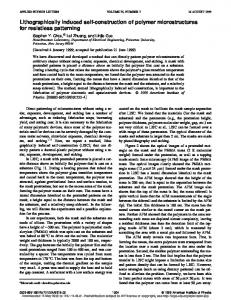
In our simulations we use the ICON data from August 17, 2000 fixed at 16:00 hours local time. The ICON sea surface temperature serves as a representative model field that we will use to motivate a glider fleet mission. ICON also supplies the flow field truth set in which the simulated gliders are advected. The ICON SST data is presented in Figure 15. The red box illustrates the area of the interest as it appears in the ICON data. Not shown are the ICON currents. For reference the depth-averaged current in that region flows predominately in a south-westerly direction.

temperature immediately below its location. More details about the data collection and the MUSE experiment can be obtained from Monterey Bay Aquarium Research Institute (MBARI)’s website [20]. Figure 14 presents the aircraft SST data. The red box illustrates a region of particular interest which corresponds to a cold tongue of water entering the bay from the north. This is characteristic of an upwelling event. In §5.3 we present simulation results of a glider fleet exploring this region. 15

70 60

14

50

13.5

13

40

degrees C

Lattitude UTM Zone 10 (km)

14.5

12.5

30 12

20 10 10

11.5

20

30

40

50

60

70

11

Longitude UTM Zone 10 (km)

Figure 14: NPS Aircraft Sea Surface Temperature, Monterey Bay, Aug. 17, 2000 Figure 15: ICON Sea Surface Temperature, Monterey Bay, Aug. 17, 2000 16:00 local time 5.1.2

Innovative Coastal-Ocean Observing Network (ICON)

5.2

The fine-resolution numerical ocean model of the Monterey Bay Area (ICON model) was developed in the “Innovative Coastal-Ocean Observing Network” (ICON) project [17]. The ICON model is a threedimensional, free surface model based on the Princeton Ocean Model (POM) [3]. The model has an orthogonal, curvilinear grid, extending 110 km offshore and 165 km in the alongshore direction. The horizontal resolution is 1-4 km with the maximum resolution in the vicinity of Monterey Bay. Vertically, the model is characterized by a realistic bottom topography with 30 vertical sigma levels. On the open boundaries the model is coupled to a larger-scale NRL Pacific West Coast model. The ICON model was run with atmospheric forcings from COAMPS (Navy Coupled Ocean and Atmospheric Mesoscale Prediction System) model predictions [8]. HF radar (CODAR)-derived surface currents are assimilated into the model [18].

Glider Simulator Details

We developed a MATLAB simulator to study the implementation of the VBAP methodologies in a practical scenario involving SLOCUM gliders used in AOSN-II. Our goal was to incorporate the operational behaviors, constraints and communication latencies of the gliders as much as possible. The glider simulator consists of two modules • Module 1 : Glider in Water - to simulate glider motion during a dive • Module 2 : Glider at Surface - to simulate glider motion (drift) when it is at the surface and to update the onboard flow estimate. 5.2.1

Glider in Water

While in water the gliders are simulated to move at a horizontal speed of 40 cm/s, and a nominal vertical 13

speed of 20 cm/s relative to water, consistent with the assumptions made in §2.1. The horizontal velocity is added to the “truth” local horizontal flow velocity, which is provided by the ICON data set, to compute the total absolute horizontal velocity of the glider. Vertical velocity from ICON model predictions was not used in this study. Instead a zero-mean white noise is added to the vertical velocity to account for the vertical component of the true local flow field The gliders are simulated to dive until 25 m above the sea floor, up to a maximum depth of 200 m. Then they move upward until they are 5 m from the surface before going downward again, unless they are surfacing in which case they go all the way to the surface. The gliders are commanded to start surfacing 2 hours after they dove into the water. Since the glider could be at any depth between 0 and 200 m when it starts surfacing, the total time of implementation of the ‘glider in water’ module will in general be a little over 2 hours during every cycle. The glider has a constant estimate of the local flow velocity, which is updated every time it surfaces and obtains a GPS fix. To calculate its absolute velocity the glider adds the local flow velocity estimate to its relative velocity (i.e., relative to water). The relative velocity is computed using the heading measurement, and the assumptions regarding the horizontal and vertical speeds. A white noise with a nonzero bias is added to the actual heading to simulate the heading sensor. The bias itself is randomly chosen at the start of every dive cycle. While in the water the glider servos its heading so that it always tries to towards the next waypoint. A three-dimensional, black-box model is used to simulate the experimentally observed input-output relation between the tailfin position (input) and the heading (output). The proportional servo controller is turned off whenever the measured heading is within a fixed deadband (±0.02 rad) of the continuously changing desired heading. A waypoint is considered reached if the horizontal distance from the waypoint is less than 25 m. 5.2.2

possible communication problems. During this time the glider also gets several GPS fixes. We use the first and the last GPS fix, and the glider’s estimate of the local flow to calculate the actual position of its surfacing. The glider corrects its flow estimate by comparing the deadreckoned and actual positions of surfacing. The corrected flow estimate is used in the computation of deadreackoned positions during the next dive. During the data exchange the glider also gets an updated set of waypoints. The glider prepares to dive after the data exchange is completed. We assume that the glider gets its last GPS fix at the end of data exchange and that it is at the surface for another minute before diving. Thus the total nominal time the glider spends at the surface is 2+17+1=20 minutes.

5.3

Preliminary and Results

Parameter

Studies

For our simulations we propose the following scenario: a perceived frontal boundary in the model data (see red box in Figure 15) motivates us to drive a fleet of gliders through this region while performing a projected gradient descent to steer the formation towards the colder regions. We assume we have a fleet of three gliders and prescribe a triangle formation since the mission entails gradient descent. During the mission, surface temperature measurements for each glider are stored along with their corresponding location. Whenever new waypoints are generated with VBAP, the last reported surface temperature measurements and corresponding locations are used to compute a least-squares gradient estimate. The gradient estimate is then used to redirect the group as described in §4. We begin the simulation with the gliders near the desired formation as shown in Figure 16. The virtual body is composed of a single virtual leader. We wish the group to head predominately south. So we choose the destination, rw , to be approximately 70 km due south from the virtual leader’s initial location. We design our artificial potentials such that the desired triangle formation about the virtual leader will be oriented such that a triangle edge spans from east to west with the inside-directed normal to that edge pointing northward. The weight w⊥ = 1. Simulations were run for approximately 12 hours. Initially we assume the fleet is synchronized and compute a VBAP plan based on each glider’s initial location. Initial local current estimates are taken to be the depth-averaged current at each glider’s location. To induce asynchronous surfacings, we artifi-

Glider at Surface

The glider is set to drift with the flow when it is on the surface. As described in §2.1, the glider does not get a GPS fix immediately after it surfaces. We assume that the first GPS fix is obtained t1 = 2 minutes after surfacing. We assume that the glider uses a nominal time of t2 = 17 minutes for exchanging data collected during the previous dive. We add a zero mean white noise with an amplitude of 2 minutes to t2 to account for 14

Figure 17: Multiple mission plans per formation cycle. Red circle indicates initial formation cen-

Figure 16: Single mission plan per formation cycle. Red circle indicates initial formation center of mass

ter of mass (virtual leader position). Tracklines denote glider trajectories. Magenta triangles illustrate glider relative locations at two hour intervals. Color contour shows “truth” sea surface temperature in degrees Celsius.

(virtual leader position). Tracklines denote glider trajectories. Magenta triangles illustrate glider relative locations at two hour intervals. Color contour shows “truth” sea surface temperature in degrees Celsius.

cially stagger the next surfacing time of each glider by 40 minutes (recall each glider surfaces approximately every 2 hours). Thus, the first glider will begin surfacing after 40 minutes, the second after 80 minutes, and the third after 120 minutes. We simulated both asynchronous implementations presented in §3.4.2. Figure 16 presents the glider trajectories when implementing a single plan per formation cycle. As shown, the fleet maintains the desired formation and detects the cold water tongue in the truth field (aircraft SST data), redirecting the fleet towards it while heading towards the destination. Figure 17 presents the glider trajectories when planning multiple times per formation cycle. The glider fleet detects the cold water tongue but does not maintain formation as well. The formation exhibits noticeable stretching and backtracking. In both instances the virtual leader is relocated to the glider formation center of mass at the start of each VBAP implementation. In Figure 18 the projected gradient weight was increased to 3 while implementing a single plan per formation cycle. As expected the group exhibits a larger deviation towards the cold water region.

Figure 18: Single mission plan per formation cycle, larger gradient weighting, w⊥ = 3. Red circle indicates initial formation center of mass (virtual leader position). Tracklines denote glider trajectories. Magenta triangles illustrate glider relative locations at two hour intervals. Color contour shows “truth” sea surface temperature in degrees Celsius.

15

6

Final Remarks

[10] N.E. Leonard and E. Fiorelli. Virtual leaders, artificial potentials and coordinated control of groups. In Proc. 40th IEEE Conference on Decision and Control, pages 2968–2973, 2001.

In this paper we have described a methodology for performing adaptive sampling using fleets of underwater gliders. We have addressed the constraints of the underwater glider, such as kinematic constraints, external currents, fleet asynchronicity, and latency, providing strategies for coping with them. We present some useful formations and strategies to perform adaptive sampling and provide detailed simulations for the purpose of both demonstration and control design validation.

[11] N.E. Leonard, J. E. Marsden, C. W. Rowley, R. Bachmayer, P. Bhatta, E. Fiorelli, F. Lekien, and S. Shadden. Proposed plan for adaptive sampling experiments in Monterey Bay ’03. http://www.princeton.edu/∼dcsl/aosn/index.html, 2003. [12] P Lermusiaux. Personal communication. 2003. [13] L. Moreau, R. Bachmayer, and N.E. Leonard. Coordinated gradient descent: A case study of lagrangian dynamics with projected gradient information. In 2nd IFAC Workshop on Lagrangian and Hamiltonian Methods for Nonlinear Control, 2003.

Acknowledgments ¨ The authors would like to thank Petter Ogren, Clancy Rowley, Ralf Bachmayer, and Rodolphe Sepulchre for their contributions to this work.

[14] P. Ogren, E. Fiorelli, and N.E. Leonard. Formations with a mission: Stable coordination of vehicle group maneuvers. In Proc. 15th International Symposium on Mathematical Theory of Networks and Systems, 2002.

References [1] http://www.princeton.edu/∼dcsl/aosn/documents/ aosn charter.doc. 2002.

[15] P. Ogren, E. Fiorelli, and N.E. Leonard. Cooperative control of mobile sensor networks: Adaptive gradient climbing in a distributed environment. Preprint, http://www.princeton.edu/∼naomi/ofl03.html, 2003.

[2] R. Bachmayer and N.E. Leonard. Vehicle networks for gradient descent in a sampled environment. In Proc. 41st IEEE Conference on Decision and Control, pages 113–117, 2002.

[16] J. Sherman, R. E. Davis, W. B. Owens, and J. Valdes. The autonomous underwater glider ‘Spray’. IEEE Journal of Oceanic Engineering, 26(4):437–446, 2001. Special Issue on Autonomous Ocean-Sampling Networks.

[3] A. Blumberg and G. L. Mellor. A description of a three-dimensional coastal ocean circulation model. Am. Geophys. Un., 4:1–16, 1987. [4] J. Cort´es, S. Mart´ınez, T. Karatas, and F. Bullo. Coverage control for mobile sensing networks: Variations on a theme. In Proc. Mediterranean Conf. on Control and Automation, 2002.

[17] I. Shulman, C. R. Wu, J. K. Lewis, J. D. Paduan, L. K. Rosenfeld, J. C. Kindle, S. R. Ramp, and C.A. Collins. High resolution modeling and data assimilation in the Monterey Bay area. Continental Shelf Research, 22:1129–1151, 2002.

[5] T. B. Curtin. AOSN-II: Monterey Bay predictive skills experiment, initial notes. May 2001.

[18] I. Shulman, C. R. Wu, J. D. Paduan, J. K. Lewis, L. K. Rosenfeld, and S. R. Ramp. High frequency radar data assimilation in the Monterey Bay. In M. L. Spaulding, editor, Estuarine and Coastal Modeling, pages 434–446, 2001.

[6] T. B. Curtin, J. G. Bellingham, J. Catipovic, and D. Webb. Autonomous oceanographic sampling networks. Oceanography, 6:86–94, 1989. [7] C. C. Eriksen, T. J. Osse, T. Light, R. D. Wen, T. W. Lehmann, P. L. Sabin, J. W. Ballard, and A. M. Chiodi. Seaglider: A long range autonomous underwater vehicle for oceanographic research. IEEE Journal of Oceanic Engineering, 26(4):424–436, 2001. Special Issue on Autonomous Ocean-Sampling Networks.

[19] H. Stommel. The Slocum mission. Oceanography, 2:22–25, 1989. [20] MBARI MUSE Data Team. MOOS upperwater-column science experiment (MUSE). http://www.mbari.org, 2001.

[8] J.C. Kindle, R. Hodur, S. deRada, J. Paduan, L. K. Rosenfeld, and F. Chavez. A COAMPS reanalysis for the Eastern Pacific: Properties of the diurnal sea breeze along the central california coast. Geophysical Research Letters, 29(24), 2002.

[21] D. C. Webb, P. J. Simonetti, and C.P. Jones. SLOCUM: An underwater glider propelled by environmental energy. IEEE Journal of Oceanic Engineering, 26(4):447–452, 2001. Special Issue on Autonomous Ocean-Sampling Networks.

[9] N. Leonard and A. Robinson. Adaptive sampling and forecasting plan. http://www.princeton.edu/∼dcsl/aosn/documents/ ASFP.pdf, 2003.

16