We also want to express our gratitude to Victor Hazlewood, Dror Feitelson and ... [Foster 1999b] I. Foster, C. Kesselman, C. Lee, R. Lindell, K. Nahrstedt, A. Roy.
Adaptive Selection of Partition Size for Supercomputer Requests Walfredo Cirne and Francine Berman Computer Science and Engineering University of California San Diego KWWS���DSSOHV�XFVG�HGX
In this paper, we show how application scheduling can be used to reduce the turn-around time of supercomputer jobs. Our approach focuses on the use of SA, an AppLeS application scheduler, to adaptively craft the request to be submitted to the supercomputer based on the current state of the system. We demonstrate that SA significantly improves a job’s turn-around time in a variety of scenarios. We also identify how the state of the system, the characteristics of the job, and the quality of the information made available to SA influence its performance.
1. Introduction In the last decade, parallel supercomputers have emerged as a key platform for high performance computation. In order to promote the performance of fine-grained parallel applications, such machines are almost always space-shared. Each job has dedicated access to some number of the processors that compose the supercomputer. We therefore say that each job runs on its own partition. In such an environment, an arriving job may not find enough processors to execute immediately. When this happens, the arriving job waits until enough resources become available. More precisely, jobs that cannot start immediately are placed in a wait queue, which is controlled by the supercomputer scheduler. The supercomputer scheduler’s main task is to decide which job in the wait queue is the next to run. In order to make this decision, it typically requires each job to specify n, the number of processors it needs, and tr, the time requested for execution of the job. However, many parallel jobs are moldable, i.e. they can run over partitions of different sizes. When a moldable job j is to be submitted, the user has to decide which n (out of the set of possible partition sizes) is to be used. The choice of n is important because it affects j’s turn-around time, i.e. the time elapsed between j’s submission and its completion. The turn-around time is calculated by adding wait time and execution time. In principle, the user is able to evaluate the effect of n on the execution time. It typically diminishes as n grows (at least until a certain value nlimit). However, the user cannot in general estimate the wait time because it depends on n, tr, the supercomputer scheduler, and the current load of the system.
1
In this paper, we introduce a performance-efficient strategy for choosing n, the number of processors a job requests. This strategy is implemented by SA (Supercomputer AppLeS). SA is an AppLeS [Berman 1996] application scheduler that adaptively crafts the request that submits a given job to the supercomputer. SA uses knowledge of how the supercomputer scheduler works, together with information that describes the current state of the system, to adaptively choose which partition size to request. We show that SA significantly improves a job’s turn-around time, and identify the factors that influence the performance achieved by SA. We also establish the maximum improvement that can potentially be achieved by adaptively selecting which request to submit to the supercomputer. Under most scenarios, SA delivers a performance improvement that is close to such a maximum. This paper is organized as follows: Section 2 describes supercomputer scheduling and the SA application scheduler. It also states the research questions we intend to address in this paper. Section 3 describes the models and metrics used to investigate these research questions. Section 4 presents and analyzes the results. Section 5 sketches directions for future research, Section 6 discusses related work, and Section 7 concludes this paper by summarizing its results.
2. Scheduling Jobs on Supercomputers In order to run a job j on a parallel supercomputer, the user submits a request to the supercomputer scheduler that specifies the resources to be allocated to j. Such a request includes n, the number of processors to be allocated to j, and tr, an upper bound on the execution time of j. Job j runs for te ≤ tr. The supercomputer scheduler kills j if it runs longer than tr, therefore enforcing the upper bound. Job j runs with dedicated access to n processors for tr time units. However, it might have to wait until such resources become available. Let tw denote the time elapsed between j’s submission and its start (i.e., the time j waits in the system’s queue). Define j’s turn-around time1 as tt = tw + te. Note that tt corresponds to the time elapsed between j’s submission and its completion. It thus captures the user’s view of how long the system takes to run j. Reducing the turn-around time tt results in faster response to the user and hence is a natural performance optimization goal. In fact, reducing tt is normally seen as a key goal for supercomputer schedulers. Here we take the complementary approach of trying to reduce the turn-around time tt at the application level. The turn-around time tt depends on the current state of the system, but it can be influenced by the request (n, tr) that submits j for execution. Jobs frequently are moldable, i.e. they can run on partitions of different sizes. This paper explores how to select which partition size to request in order to improve a moldable job’s turn-around time. The execution time te generally decreases with the number of processors n allocated to the job. Of course each job has a limit nlimit of how many processors it can effectively use, i.e. te levels off or even increases for n > nlimit. But since there is no advantage in requesting n > nlimit, we don’t consider such requests here. Note that increasing n might result in a larger wait time tw, because more resources have to be available for the job to
1
Other authors sometimes refer to turn-around time as service time or response time.
2
start. Since tw depends on the current state of the supercomputer, the best request to submit cannot be statically determined. We use SA (Supercomputer AppLeS) to select which n (and corresponding tr) should be used to submit a moldable job to the supercomputer. SA is based on the AppLeS (Application-Level Scheduling) methodology [Berman 1996] [Berman 1997]. AppLeS schedulers use application-specific and dynamic information to craft an adaptive application schedule that can leverage current and forecasted resource capability. SA determines the partition size n to be requested based information about the algorithm used by the supercomputer scheduler, the current state of the system, and estimates for the execution times of all jobs in the system. Using this information, SA simulates the submission of all possible requests and then selects the one that delivers the smallest turn-around time. When (i) the execution time estimates of all jobs are perfect, and (ii) the supercomputer scheduler does not allow arriving jobs to affect existing ones, this approach optimally selects the partition size for a given job. However, while assumption (ii) may be true, in practice assumption (i) is not. SA uses requested times as estimates for the jobs’ execution times, making it usable in practice, but without the guarantee of optimality. This work investigates, under common supercomputer usage scenarios: • The performance achieved by SA. • The maximum improvement that can be achieved by adaptively selecting the partition size. • What factors influence SA and the maximum improvement.
3. Models and Metrics We use simulations to tackle the questions stated above. This section describes (i) the models used for the supercomputer and the job, (ii) the information made available to SA, and (iii) our performance criteria. Our goal is to reproduce a realistic environment, while capturing enough detail to answer our research questions. To ensure the realism of the environment, we rely as much as possible on real-life submission logs.
3.1. The Supercomputer Model In order to simulate a supercomputer, we need to define its scheduler, its size (how many processor it has), and its workload (the stream of jobs it is going to process). Consider a supercomputer that uses conservative backfilling [Feitelson 1998a]. Conservative backfilling uses an allocation list to maintain, for any given time, which processors are already committed to which jobs. Arriving jobs are put in the first “slot” in which they fit. Whenever an application finishes using less time than it requested, conservative backfilling traverses the wait queue (in submission order) and “promotes” the first job that fits in the just-made-available slot. Of course, this may create another available slot that is backfilled in the same way. The process stops only when no more backfilling can be done. For a more detailed description of conservative backfilling, we refer the reader to [Feitelson 1998a] and [Cirne 1999]. We employ conservative backfilling as an idealized representative of today’s supercomputer schedulers. In practice the behavior of supercomputer schedulers varies from machine to machine. Even when the same scheduling software is used (e.g., Easy [Lifka 1995], Maui [Maui], and LSF [Platform]), each site establishes its own policies, 3
causing the behavior of their schedulers to differ. However, almost everywhere backfilling is used to reduce unnecessary idle time. In addition, previous research has shown conservative backfilling to be a good scheduling approach [Feitelson 1998a]. Note also that conservative backfilling guarantees that arriving jobs don’t affect existing ones. The state of a conservative backfilling scheduler can be summarized by the availability list. An availability list contains the number of free processors a machine has over time. For example: >�IURP�WLPH����WR�WLPH��������SURFHVVRUV�DUH�DYDLODEOH ���IURP�WLPH�����WR WLPH� ���� ��� SURFHVVRUV� DUH� DYDLODEOH �� �IURP� WLPH� ���� WR� WLPH� ����� �� SURFHVVRUV� DUH� DYDLO� DEOH ���IURP�WLPH������WR�
∞������SURFHVVRUV�DUH�DYDLODEOH @. The availability list allows for a
very fast implementation of SA, which doesn’t simulate all possible requests to choose the best, but achieves the same result. Such an implementation evaluates all possible requests by traversing the availability list. Due to space limitations and the fact that both implementation of SA produce the same result, we refer the reader to [Cirne 1999] for a thorough description of SA based on the availability list. For the size of the supercomputer and the workload it processes, we use the size of real-life supercomputers as well as the logs of the jobs submitted to them. We decided to use logs because supercomputer behavior is difficult to characterize [Downey 1999]. The drawback of this approach is that we might be misled by some phenomenon that is particular to the site a log originates. We minimize this risk by using four distinct supercomputer logs. The following table summarizes the logs used in this research. The fact that all logs come from an SP2 machine is not significant. The results presented here would apply to any distributed-memory parallel computer that serves multiple users via space-sharing. Name Machine ANL
Argonne National Laboratory SP2 CTC Cornell Theory Center SP2 KTH Swedish Royal Institute of Technology SP2 SDSC San Diego Supercomputer Center SP2
Processors
Jobs
Period
120
5921 Nov 1996 Dec 1996 430 60196 Jul 1996 Feb 1997 100 25954 Nov 1996 Aug 1997 128 19405 Jan 1999 May 1999
Table 1 – Workloads used in this research SA makes its scheduling decisions based on the current state of the system, and thus we expect the system state to influence the performance it achieves. We summarize the state of the supercomputer by its relative load N = J / P, where J is the number of jobs currently in the system (both running and waiting), and P is the total number of processors in the supercomputer (see Table 1). J is a simple way to gauge the load of the supercomputer. Dividing it by P factors in the size of the supercomputer.
3.2. The Job Model SA targets moldable jobs. For each job it schedules, SA receives from the user multiple requests that could be used to submit the job. From the set of possible requests, SA determines which is the best one to submit according to the current state of the
4
supercomputer. Unfortunately for our study, the submission logs contain only one request per job (namely, the one submitted by the user). We cope with this limitation by using a model of the speed-up of parallel jobs developed by Downey [Downey 1997a]. Speed-up measures how much faster a job j that uses n processors executes than execution using only one processor. Symbolically: S(n) = te(1) / te(n). If we know the speed-up function S(n) for our jobs, we can generate multiple possible requests for them. Downey’s speedup model uses two parameters: A (the average parallelism) and σ (an approximation of the coefficient of variance in parallelism). The speed-up of a job is then given by: An R | A + V (n − 1) / 2 | An | |V ( A − 1 / 2) + n(1 − V / 2) S ( n , A, V ) = S A | nA(V + 1) | | V (n + A − 1) + A | | A T
(V ≤ 1) ∧ (1 ≤ n ≤ A) (V ≤ 1) ∧ ( A ≤ n ≤ 2 A − 1) (V ≤ 1) ∧ (n ≥ 2 A − 1) (V ≥ 1) ∧ (1 ≤ n ≤ A + AV − V ) (V ≥ 1) ∧ (n ≥ A + AV − V )
Intuitively speaking, A establishes how many processors a job can use. The larger the value of A, the more processors the job can use. Figure 1 exemplifies how A affects the speed-up of a job. It fixes σ = 1 and shows speed-up curves for different values of A. Downey’s speed−up for different values of A (σ = 1) 100 A = 100 A = 80 A = 60 A = 40 A = 20
90
80
70
Speed−up
60
50
40
30
20
10
0
0
20
40
60
80 100 120 Number of Processors
140
160
180
200
Figure 1 – Downey’s speed-up function S(n, A, σ) for different values of A (with σ = 1)
5
σ, on the other hand, determines how close to linear the speed-up is. The smaller the σ, the closer to linear the speed-up is. Figure 2 explores the effect of σ on the speedup behavior. It fixes A = 60 and displays speed-up curves for different values of σ. Downey’s speed−up for different values of σ (A = 60) 70
60
Speed−up
50
40
30
20 sigma = 0 sigma = 0.5 sigma = 1 sigma = 2 sigma = ∞
10
0
0
20
40
60
80 100 120 Number of Processors
140
160
180
200
Figure 2 – Downey’s speed-up function S(n, A, σ) for different values of σ (with A = 60) Since we are interested in understanding the performance of SA in a variety of conditions, we vary the values of A and σ. We uniformly choose A in the interval [2, 200] and σ in the interval [0, 2]. This gives large coverage over a wide range of parallel jobs. Moreover, experimental determination of values for A and σ have produced values in these ranges [Downey 1997a]. From the workload we can obtain nu, the number of processors requested by the user, and te(nu), the job’s execution time with nu processors. Note that A, σ, nu, and te(nu) uniquely determine the sequential execution time of the job L = te(1) = te (nu ) ⋅ S (nu , A, V ) . L represents how “large” a job is. The greater the L, the more processing is required to complete the job. With A, σ and L, we can determine the execution time of the job running over an L . A, σ, and L therefore characterize arbitrary number of processors n by te (n) = S (n, A, V ) the job being scheduled by SA.
3.3. Information Available to SA Many jobs have constraints on how many processors they can use. For example, jobs that process bidimensional data many times require a perfect square number of processors. Moreover, the user has to come up with the submission choices to feed SA. These factors suggest that oftentimes SA will have only a small number of choices to choose
6
from. Therefore, we focus on the cases in which jobs are presented to SA with 3, 5, or 7 possible requests. Another important aspect of the information available to SA is how far apart the choices are. Considering possible partition sizes of 40, 41, and 42 may be very different than having 10, 40, and 70. Hence we also investigate the impact of the range of choices on SA. We consider choices equally spaced in the range [nmin, nmax], where nmin is uniformly chosen between 1 and nu, and nmax is uniformly chosen between nu and nlimit. nlimit is the largest number of processors a job can use, defined to be the smaller of (i) the number of processors in the machine, and (ii) the largest n before the Downey’s speed up curve levels off. Finally, accuracy represents a qualitative aspect of the information SA receives. Users’ estimates are not perfect. We define the accuracy a as the fraction of the requested time that was indeed used by a job. That is, a = te / tr. Since jobs cannot run longer then the time they’ve request, a is always a number between 0 and 1. In our simulations, a is uniformly distributed between 0 and 1, allowing us to investigate the impact of both good and poor information. The number of choices, the size of their range (nmax – nmin), and the accuracy a are the factors that characterize the information made available to SA.
3.4. The Performance Criteria Turn-around time is a useful metric for a single execution of a job. However multiple executions are necessary to draw statistically valid conclusions, as well as to cover the space of parameters we are investigating. Hence, we need a performance metric that summarizes turn-around times over multiple experiments. Many researchers have used the mean to combine multiple turn-around times into a single metric [Aida 1998] [Cirne 1999] [Feitelson 1998b] [Krallmann 1999]. However, the mean turn-around time can be dominated by large jobs [Feitelson 1998b]. For example, improving a job’s turn-around time from 20000 seconds to 18000 seconds (a 10% improvement) reduces the mean by 2000 / T, while improving another job’s turn-around time from 200 seconds to 100 seconds (a 50% improvement) reduces the mean by 100 / T, where T is the total number of jobs. Some authors have addressed this problem by using the slowdown s = tt / te instead of the turn-around time [Feitelson 1998a] [Feitelson 1998b] [Zotkin 1999]. Slowdown provides a measure that is relative to the job’s execution time and hence large jobs are not overemphasized in the mean slowdown. However, slowdown is not a metric that adequately represents the user’s notion of performance. In our case, in which there are multiple possible requests to submit, one can often improve the slowdown by selecting nmin. This results in a large te, which often leads to a small slowdown s. The problem is that such a strategy can (and often does) increase the turn-around time. The geometric mean equally rewards the improvement in the turn-around time of geomean( x1 ,..., xn ) any job. In fact, recall that geomean( x1 ,..., xn ) = n x1 ⋅...⋅ xn and thus geomean( y1 ,..., yn ) x1 xn = geomean( ,..., ) . Unlike the arithmetic mean, the geometric mean does not favor y1 yn large jobs. For this reason, the geometric mean is used to aggregate the execution time of
7
the programs that compose the Spec benchmark [SPEC]. We hence use the geometric mean of the turn-around times as our performance criteria.
4. Results We ran 56000 simulations: 14000 per workload. In each simulation, we randomly chose one job j, generated A, σ, nmin, nmax, and a as described above, and simulated five strategies for submitting j: i. Using the user’s request, i.e. without SA. ii. Using SA with 3 choices for partition sizes. iii. Using SA with 5 choices for partition sizes. iv. Using SA with 7 choices for partition sizes. v. Best choice, i.e. we simulate the submission of all 7 choices offered to SA and report the best turn-around time among them. While it is not generally possible to determine the best choice in practice, strategy v establishes the best performance SA can achieve in our experiments, offering a bound on the maximum improvement achievable by adaptively crafting requests to a supercomputer. In order to better assess the maximum improvement, we define the relative performance for strategies ii to v as the ratio of the turn-around obtained by the user’s request to the turn-around time achieved the strategy in consideration. The relative performance depicts how many times SA improved on the turn-around time. In particular, the relative performance of the best choice expresses the maximum improvement possible in our experiments. Table 2 shows the overall results for the 56000 simulations. Notice the high maximum improvement of adaptively selecting supercomputer requests: The turn-around time of best choice is around a third of the turn-around time attained by the user’s choice, yielding a relative performance of 2.98. Furthermore, SA is able to deliver turn-around times close to the best choice: With 7 choices, SA’s relative performance reaches 2.78. Even with 3 choices, SA delivers a substantial improvement: Its turn-around time is less than half of the turn-around time of user’s choice.
Geometric Mean of the Turn-Around Time (secs) Relative Performance
User’s SA with SA with SA with Best choice 3 choices 5 choices 7 choices choice 1259.9 600.2 525.3 453.3 423.6 -----
2.10
2.40
2.78
2.98
Table 2 – SA overall results In the following subsections, we investigate how SA and the maximum improvement are affected by the various parameters that describe the system, the job, and the information received by SA.
4.1. Results by the State of the System Figure 3 shows the impact of the relative load N on the results. The experiments are grouped in deciles according to N. Therefore, each data point in the graph averages around 5600 experiments. The values of N on the x-axis show the boundaries of the deciles. That is, the values that surround a given data point establish the range of values
8
averaged by such a point. Unless stated otherwise, the following graphs display the data in the same way. 5 User’s choice SA with 3 choices SA with 5 choices SA with 7 choices Best choice
4500 4000 3500 3000 2500 2000 1500
SA with 3 choices SA with 5 choices SA with 7 choices Best choice
4.5
Relative Performance
Geometric Mean of Turn−Around Time
5000
4 3.5 3 2.5 2
1000 1.5
500 0
0
.04 .06 .07 .09 .11 .14 .17 .23 .33 3.5 N
1
0
.04 .06 .07 .09 .11 .14 .17 .23 .33 3.5 N
Figure 3 – Results by N, the relative load of the system As expected, the turn-around time increases with N. This is because the more jobs there are in the system, the longer an arriving job has to wait in the queue. The relative performance provides a less intuitive result. It decreases as N increases for both best choice and SA. This suggests that adaptively selecting which request to submit becomes less useful as the load in system grows.
4.2. Results by Characteristics of the Job The job scheduled by SA can be characterized by three parameters: the sequential execution time L, the average parallelism A, and the coefficient of variance in the parallelism σ. Recall that L measures the amount of computation j carries, A indicates how many processors j can effectively use, and σ denotes the slope of j’s speed-up (the closer σ is to 0, the closer to linear the speed-up is). Figure 4, Figure 5, and Figure 7 show how such parameters affect the performance of SA and the maximum improvement achieved by adaptively generating requests. As one can expect, the larger the L (i.e., the more computation a job carries), the greater the turn-around time. But the wide distribution of L makes it hard to visualize any other patterns in the turn-around time graph. Relative performance provides a more insightful picture. Notice that the relative performance decreases for large values of L, those in 10th decile. For those jobs, the execution time represents a large fraction of the turn-around time, giving less latitude for SA to improve the job’s performance. Consequently, one would think that the greatest relative performance must occur for small values of L. Somewhat surprisingly, however, this is not the case. As can be seen in the graph, medium values of L (say in the [2000, 50000] range) provide the best relative performance. A closer look at the jobs with small L reveals that most of them have very small turn-around times (up to 300 seconds). We conjecture that small jobs are easier to schedule in the presence of backfilling and thus get through the system quickly, mini-
9
mizing the benefits of SA. Another interesting result is that the smaller the L, the more advantageous it is to have more choices. We are not sure why that is the case. 4
x 10
4.5 User’s choice SA with 3 choices SA with 5 choices SA with 7 choices Best choice
4 3.5
SA with 3 choices SA with 5 choices SA with 7 choices Best choice
4
Relative Performance
Geometric Mean of Turn−Around Time
4.5
3 2.5 2 1.5
3.5 3 2.5 2
1 1.5
0.5 0
0
142
776
6048
1
40872 6976561
0
142
776
L
6048
40872 6976561
L
Figure 4 – Results by L As Figure 5 shows, the larger the A (i.e., the greater the potential for parallelism in the job), the greater the relative performance achieved by SA and the best choice. This behavior seems reasonable because the greater the average parallelism A, the more flexibility SA has in selecting a good request, which translates to a greater improvement in the job’s turn-around time. Also, the utility of having more choices available to SA grows with A. 3.6 SA with 3 choices SA with 5 choices SA with 7 choices Best choice
3.4 1200
3.2
1000 User’s choice SA with 3 choices SA with 5 choices SA with 7 choices Best choice
800
600
Relative Performance
Geometric Mean of Turn−Around Time
1400
3 2.8 2.6 2.4 2.2 2
400
1.8 200
0
22
42
62
82 100 120 140 160 180 200 A
1.6
0
22
42
62
82 100 120 140 160 180 200 A
Figure 5 – Results by A Note that in these experiments the increase in the relative performance slows down for A ≥ 100. Similarly, the benefit of having more choices available to SA grows slower for A ≥ 100. We believe this is related to the fact the three out of the four supercomputers we simulated have only slightly more processors than this value (see
10
2000
6.5
1800
6
1600
5.5
Relative Performance
Geometric Mean of Turn−Around Time
Table 1). To expand on this, consider the CTC results in isolation (the SP2 used there had 430 nodes), as shown in Figure 6. As can be seen, the relative performance keeps increasing steadily beyond A = 100.
1400 User’s choice SA with 3 choices SA with 5 choices SA with 7 choices Best choice
1200 1000 800
5 4.5 4 3.5
600
3
400
2.5
200
0
22
42
62
2
82 100 120 140 160 180 200 A
SA with 3 choices SA with 5 choices SA with 7 choices Best choice
0
22
42
62
82 100 120 140 160 180 200 A
Figure 6 – CTC results by A The results by the coefficient of variance of parallelism σ are very surprising. As Figure 7 shows, SA seems to be completely indifferent to σ. We expected SA to perform better with smaller values of σ since these imply a speed-up closer to linear. Further investigations are required to determine why SA exhibits such robust performance regarding σ.
SA with 3 choices SA with 5 choices SA with 7 choices Best choice
1300 1200
Relative Performance
Geometric Mean of Turn−Around Time
1400
1100 User’s choice SA with 3 choices SA with 5 choices SA with 7 choices Best choice
1000 900 800 700
3
2.5
600 500 400
0
0.2 0.4 0.6 0.8
1 σ
1.2 1.4 1.6 1.8
2
2
0
0.2 0.4 0.6 0.8
1 σ
1.2 1.4 1.6 1.8
2
Figure 7 – Results by σ
4.3. Results by Information Available to SA The information made available to SA also impacts its performance. We characterize the amount and quality of such information by (i) the number of choices available
11
1600
3.2
1400
3
1200
2.8
Relative Performance
Geometric Mean of Turn−Around Time
to SA, (ii) the size of the range of such choices, and (iii) the accuracy of the users’ estimates a. The number of choices available to SA is an especially important parameter because this information must be provided by the user. We therefore treated the number of choices independently of the other simulation parameters. This allows for the evaluation of the impact of the number of choices as a function of the other parameters. Figure 3 through Figure 9 present our results. Figure 8 contains the results by a, the accuracy of the users’ estimates. Recall that a = te / tr. Therefore a small a implies that the request asked for much more time than the job actually used. Note that a large request is harder to fit in the availability list and also harder to backfill (compared to a smaller one). We thus expected a to strongly impact the results. However, a shows almost no impact on the maximum improvement and little impact on the performance actually attained by SA. While it is true that small values of a (say a ≤ 0.2) result in greater turn-around times for all strategies, we expected this to happen more intensely. Similarly, very small values of a (say a ≤ 0.1) reduce the relative performance of SA, but again to a lesser degree than we expected. Our results seem to corroborate other studies that have found inaccurate user’s estimates not to significantly hurt performance [Feitelson 1998a] [Zotkin 1999].
User’s choice SA with 3 choices SA with 5 choices SA with 7 choices Best choice
1000 800 600 400 200
2.6 2.4 2.2
SA with 3 choices SA with 5 choices SA with 7 choices Best choice
2
0
0.1 0.2 0.3 0.4 0.5 0.6 0.7 0.8 0.9 a
1
1.8
0
0.1 0.2 0.3 0.4 0.5 0.6 0.7 0.8 0.9 a
1
Figure 8 – Results by a (accuracy of the requests) Figure 9 shows results by varying the size of the range of choices. As before, the results were grouped into deciles. However, 29.2% of the experiments had range size equals 7 (this happened so often because many jobs have small nu or nlimit). For that reason, the first data point in the graph averages the first three deciles of experiments, and the graphs contain seven data point instead of ten. As expected, the maximum improvement grows with the size of the range. The greater the size of the range, the more leverage SA has in finding a good request to submit. In particular, large ranges (say above 100) seem to provide a substantial boost in the relative performance of both SA and best choice.
12
5.5
1400
5
1200
Relative Performance
Geometric Mean of Turn−Around Time
1600
User’s choice SA with 3 choices SA with 5 choices SA with 7 choices Best choice
1000 800 600
4.5 4 3.5 3 2.5
400 200
SA with 3 choices SA with 5 choices SA with 7 choices Best choice
2
0
13
25
37 49 61 73 Range of Choices
91
367
1.5
0
13
25
37 49 61 73 Range of Choices
91
367
Figure 9 – Results by the size of the range of choices
4.4. Simulations Using Real Speedups Simulations are an important research tool. They allow us to explore issues that are not tractable analytically or experimentally. However, they can produce invalid results due to a number of reasons, from poor modeling of reality to undetected bugs in the simulator. Consequently, it is important to double-check the results obtained via simulations. A crucial part of our simulation model is the job speedup function. In this Section, we show the results of experiments designed to investigate whether using the Downey’s model of parallel speed-up skewed our results. For these experiments, we used NAS benchmarks (which have known speed-up behavior) as the jobs to be scheduled by SA. NAS benchmarks have known execution times for a variety of supercomputers and partition sizes. Such data is publically available at . Moreover, since they are used to evaluate performance, they are representative of real jobs. Finally, some of the NAS benchmarks are constrained with respect to the number of processors they can use. For some, the number of processors must be a perfect square. For others, it must be a power-of-two. This represents another real-world constraint for SA. In the experiments, we replaced one job in the workload by a NAS benchmark (which has known speed-up). We then compared the performance of this NAS benchmark (i) when SA decides which request to submit, versus (ii) when we request the same number of processors for the NAS benchmark as the job we replace. We use five NAS benchmarks: MG, LU, SP, BT, and EP. MG and LU require a power-of-two partition size � contains and thus are the most constrained jobs. execution time information of MG and LU over 8, 16, 32, 64, 128, and 256 processors for the SP2. Consequently, for MG and LU, SA had 4 to 6 choices depending on the number of processors of the supercomputer being used (see Table 1). SP and BT require perfectsquare partition size. The execution time data contains information for 9, 16, 25, 36, 64, 121, and 256 processors; providing 5 to 7 choices available to SA. There are no restrictions for EP. It can run over any number of processors and thus there are as many choices KWWS���ZZZ�QDV�QDVD�JRY�6RIWZDUH�13%�
KWWS���ZZZ�QDV�QDVD�JRY�6RIWZDUH�13%�
13
as processors in the supercomputer. We performed 10000 simulations in total: 2000 per NAS benchmark. Table 3 shows the overall results of using NAS benchmarks as the job SA schedules. The results are consistent with those found when Downey’s model is used to generate speed-up information (see Table 2). As before, SA gets relatively close to results obtained by the best choice. Furthermore, SA improves the turn-around time of the NAS benchmarks by a factor of 4.19 compared to the user’s choice, a result even better than the one achieved using Downey’s model. We attribute this better performance to the fact that EP provides SA with many more choices than what we have been considering (up to 7 choices), creating the opportunity for an even greater improvement in performance. User’s choice SA choice Best Choice 1164.70 278.04 253.05
Geometric Mean of the Turn-Around Time (secs) Relative Performance
-----
4.19
4.60
Table 3 – Overall NAS results Indeed, consider Figure 10, which groups the results by the restriction posed by the number of processors a NAS benchmark can use. Note that the maximum improvement is greater for EP than for the other NAS benchmarks. The presence of EP also explains the greater maximum improvement of NAS benchmarks (whose best choice’s relative performance equals 4.60) compared to jobs with Downey’s speed-up (whose best choice’s relative performance equals 2.98). The large number of choices offered by EP makes adaptively selecting the request more attractive. Note also that SA is still able remain close to the maximum improvement for EP, which suggests that increasing the number choices doesn’t make it harder for SA to find a very good request. 10 User’s choice SA choice Best choice
9
2000
8
Relative Performance
Geometric Mean of Turn−Around Time
2500
1500
1000
500
7 SA choice Best choice
6 5 4 3 2 1
0
LU/MG
BT/SP NAS Benchmark
EP
0
LU/MG
BT/SP NAS Benchmark
EP
Figure 10 – NAS results by kind of benchmark Figure 11 contains the NAS results by N, the relative load of the system. As with the simulations based on Downey’s speedup (see Figure 3), the execution time increases with N. Again, this is because the more jobs there are in the system, the longer an arriving job will probably have to wait in the queue. The relative performance, on the other hand, 14
tends to decrease as N increases, showing however a modest increase for N ≥ 0.2. Since the relative performance for jobs with Downey’s speed stabilizes around the same value, we don’t believe this represents a distinct phenomenon. 6.5 User’s choice SA choice Best choice
10000
SA choice Best choice
6 5.5
Relative Performance
Geometric Mean of Turn−Around Time
12000
8000
6000
4000
5 4.5 4 3.5 3
2000 2.5 0
0
2
.04 .06 .07 .09 .11 .14 .17 .23 .33 3.5 N
0
.04 .06 .07 .09 .11 .14 .17 .23 .33 3.5 N
Figure 11 – NAS results by N (number of jobs in the system) Figure 12 presents the results by the accuracy of the user’s estimates a. Note the similarity to Figure 8, which displays the results based on Downey’s model by accuracy. Again SA presents a high tolerance to variance in accuracy a. Only small values of a seem to affect the performance of SA. 4.2 User’s choice SA choice Best choice
1800
SA choice Best choice
4
1600
Relative Performance
Geometric Mean of Turn−Around Time
2000
1400 1200 1000 800
3.8 3.6 3.4 3.2
600 3
400 200
0
0.1 0.2 0.3 0.4 0.5 0.6 0.7 0.8 0.9 a
1
2.8
0
0.1 0.2 0.3 0.4 0.5 0.6 0.7 0.8 0.9 a
1
Figure 12 – NAS results by a (accuracy of the requests) We therefore believe that the NAS results validate the use of Downey’s model in our simulations.
15
5. Future Work As with any research, this answers some questions but raises others. To follow up this work, there are four research topics we intend to pursue. First, we would like to develop SA into a tool for production jobs. For some sites, the supercomputer scheduler allows for arriving jobs to affect existing ones, increasing the uncertainty SA has to cope with. It would be important to evaluate the impact of this added uncertainty on SA. Second, we intend to investigate the effect multiple instances of SA have on each other, a question that has been called the Bushel of AppLeS [Berman 1997]. We expect the improvements to the performance of an individual job to be smaller when many jobs have their requests crafted by SA, because the system as whole becomes more efficient, making it harder for SA to find very good “slots” in the supercomputer schedule. We want to investigate whether this is really the case and, if so, to what extent. Also, it might be that different mixtures of jobs produce different Bushel of AppLeS effects. This also needs to be understood. Third, we plan to extend SA to target multiple supercomputers, instead of only one. In principle, SA could be used to submit the same job to all available supercomputers. While this guarantees a turn-around time that is at least no worse than selecting one supercomputer, it increases the load on all supercomputers, and thus might produce a bad Bushel of AppLeS effect. If this indeed happens, it is natural to ask what policies can supercomputer schedulers implement to discourage such a submit-to-all strategy. For example, charge for submission as well as execution might be a promising approach. Fourth, we aim to enable SA to better deal with priorities. Real-life supercomputer schedulers enable users to specify a priority to the jobs they submit. SA could deal with priorities at the cost of spending more time scheduling. However, it is very plausible that some users don’t want to optimize for turn-around time at any cost. How we enable the user to express an optimization goal that includes cost and how SA pursues such a goal are also intriguing research questions.
6. Related Work There has been great interest in supercomputer scheduling in recent years. Some of the research in this area allow for the scheduler to choose the number of processors allocated to a job [Downey 1997b] or even to change this number during the execution of the job [Chiang 1996] [Nguyen 1996]. Such schedulers therefore try to improve the performance of the system in the same way SA aims to improve the performance of the job. The main distinction is exactly that these efforts take the system-wide viewpoint. Alternatively, we approach the problem by scheduling one job at a time and use a user-centric performance metric. The very fact the SA works at the application level, makes it potentially useful for Grid Computing [Foster 1999a]. Computational Grids consist of resources that are geographically scattered and/or under control of multiple entities, but can be combined as execution platform for some application. In this scenario, one needs an application scheduler to select the resources of interest, determine what piece of work is to be assigned to each to them, and then craft requests to have each piece of work carried out. This applicability of SA to Grid Computing is no accident. In fact, it was instrumental in
16
deciding for the application-level approach (in opposition to the system-level one). As mentioned in the previous Section, we plan to extend SA to deal with multiple supercomputers, potentially by selecting which machine to submit the job to. The current research in Grid scheduling that involves supercomputers seems to target jobs that spread across multiple machines. Advance reservations are the basic service to support application scheduling for such jobs [Chapin 1999] [Foster 1999b]. They have been shown to provide better system-wide utilization compared to dedicating supercomputer time for the jobs that spread across multiple supercomputers [Snell 1999]. Interestingly enough, the availability list is touted in this context as providing the information that enables one to decide on which reservation to request [Chapin 1999] [Foster 1999b] [Nitzberg 1999]. Our research complements this work in that it explores the availability list to improve the performance of jobs that use a single supercomputer, a far more common case. An alternative approach was adopted by the GTOMO, a Grid application that simultaneously uses supercomputer nodes and workstations [Smallen 2000]. GTOMO relies on a simplified version of the availability list to craft a request that can start running immediately. GTOMO can use this strategy because it schedules an embarrassingly parallel application, which can always start running immediately on the workstations. The supercomputer processors that happen to be available simply add more resources to the poll of workstations, boosting therefore the performance of the application.
7. Conclusions This paper demonstrates that adaptively selecting the partition size of a supercomputer request can substantially improve the job’s turn-around time. Here we introduce SA, an AppLeS application scheduler, and evaluate how it performs with four different real-world workloads. SA schedules moldable jobs, i.e. jobs that have flexibility regarding the size of the partition on which they execute. It decides which partition size should be requested considering the current state of the system, and consistently improves the turn-around time compared to the user’s choice. We simulate SA with four different workloads to evaluate how it performs under a variety of scenarios. We found SA to consistently improve the turn-around time of the job it schedules, but by different degrees depending on the scenario. In summary, the performance improvement attained by SA improves with the increase in the amount of parallelism in the job, the number of choices SA has available to choose from, and the range over which such choices are spread. On the other hand, SA’s performance decreases with the system’s load. The size of the job doesn’t appear to have a linear correlation to the performance of SA: SA does better for medium sized jobs than for small or large jobs. Finally, the slope of the job’s speed-up and the accuracy of the user’s estimates seem to have surprisingly little effect on SA. We also investigate how close SA gets to the turn-around time obtained by the best choice offered to it. Always finding the best choice is impossible in practice due to the lack of perfect information about the jobs’ execution times. Nevertheless, we found SA’s performance to be close to (above 90% of) the performance achieved by the best choice.
17
Acknowledgments We thank our supporters: CAPES grant DBE2428/95-4, DoD Modernization contract 9720733-00, NPACI/NSF award ASC-9619020, and NSF grant ASC-9701333. We also want to express our gratitude to Victor Hazlewood, Dror Feitelson and the people who made their workloads available at the Parallel Workloads Archive (KWWS���ZZZ�FV�KXML�DF�LO�ODEV�SDUDOOHO�ZRUNORDG�). Finally, thanks to the members of the AppLeS group, Rich Wolski, Allen Downey, and Warren Smith for the insightful discussions and valuable suggestions.
References [Aida 1998]
[Berman 1996]
Kento Aida, Hironori Kasahara, and Seinosuke Narita. Job Scheduling Scheme for Pure Space Sharing among Rigid Jobs. In Job Scheduling Strategies for Parallel Processing, Springer-Verlag, Lecture Notes in Computer Science Vol. 1459. Fran Berman, Richard Wolski, Silvia Figueira, Jennifer Schopf, and Gary Shao. Application-Level Scheduling on Distributed Heterogeneous Networks. Supercomputing’96. KWWS���ZZZ�FVH�XFVG�HGX�JURXSV�KSFO�DSSOHV�KHWSXEV�KWPO
[Berman 1997]
Fran Berman and Rich Wolski. The AppLeS Project: A Status Report. In Proceedings of the 8th NEC Research Symposium, Berlin, Germany, May 1997. KWWS���ZZZ�FV�XFVG�HGX�JURXSV�KSFO�DSSOHV�KHWSXEV�KWPO
[Cirne 1999]
Walfredo Cirne and Fran Berman. Application Scheduling over Supercomputers: A Proposal. UCSD-CS99-631 Technical Report, October 1999. KWWS���ZZZ�FV�XFVG�HGX�5HVHDUFK�7HFK5HSRUWV�GLHQVW�KWPO
[Chapin 1999]
Steve J. Chapin, Dimitrios Katramatos, and John Karpovich. The Legion Resource Management System. IPPS Workshop on Job Scheduling Strategies for Parallel Processing, pp. 105-114, San Juan, Puerto Rico, 1999. KWWS���ZZZ�FV�YLUJLQLD�HGX�aFKDSLQ�SDSHUV�DOOSXE�KWPO
[Chiang 1996]
Su-Hui Chiang and Mary K. Vernon. Dynamic vs. Static QuantumBased Parallel Processor Allocation. In Job Scheduling Strategies for Parallel Processing, Springer-Verlag, Lectures Notes in Compututer Science vol. 1162, pp. 200-223, 1996. KWWS���ZZZ�FV�ZLVF�HGX�aVXKXL�VXKXL�KWPO
[Downey 1997a] Allen B. Downey. A model for speedup of parallel programs. U.C. Berkeley Technical Report CSD-97-933. KWWS���ZZZ�VGVF�HGX�aGRZQH\�PRGHO�
[Downey 1997b] Allen B. Downey. Using Queue Time Predictions for Processor Allocation. In Job Scheduling Strategies for Parallel Processing, SpringerVerlag, Lect. Notes Comput. Sci. vol. 1162, 1997. KWWS���ZZZ�VGVF�HGX�aGRZQH\�SUHGDOORF�
18
[Downey 1999]
A. B. Downey and D. G. Feitelson. The elusive goal of workload characterization. Perf. Eval. Rev. 26(4), pp. 14-29, Mar 1999. KWWS���ZZZ�FV�KXML�DF�LO�aIHLW�SXE�KWPO
[Feitelson 1998a] D. G. Feitelson and A. Mu'alem Weil. Utilization and predictability in scheduling the IBM SP2 with backfilling. In 12th Intl. Parallel Processing Symp., pp. 542-546, April 1998. KWWS���ZZZ�FV�KXML�DF�LO�aIHLW�SXE�KWPO
[Feitelson 1998b] D. G. Feitelson and L. Rudolph. Metrics and benchmarking for parallel job scheduling. In Job Scheduling Strategies for Parallel Processing, pp. 1-24, Springer-Verlag, 1998. Lecture Notes in Computer Science Vol. 1459. KWWS���ZZZ�FV�KXML�DF�LO�aIHLW�SXE�KWPO
[Foster 1999a] [Foster 1999b]
Ian Foster and Carl Kesselman (editors). The Grid: Blueprint for a New Computing Infrastructure. Morgan Kaufmann Publishers. 1999. I. Foster, C. Kesselman, C. Lee, R. Lindell, K. Nahrstedt, A. Roy. A Distributed Resource Management Architecture that Supports Advance Reservations and Co-Allocation. International Workshop on Quality of Service, 1999. KWWS���ZZZ�IS�JOREXV�RUJ�GRFXPHQWDWLRQ�SDSHUV�KWPO
[Krallmann 1999] Jochen Krallmann, Uwe Schwiegelshohn, and Ramin Yahyapour. On the Design and Evaluation of Job Scheduling Algorithms. In Job Scheduling Strategies for Parallel Processing, Springer-Verlag, Lectures Notes in Compututer Science vol. 1659, 1999. [Lifka 1995] David Lifka. The ANL/IBM SP Scheduling System. In Job Scheduling Strategies for Parallel Processing, D. G. Feitelson and L. Rudolph (Eds.), Springer-Verlag, Lecture Notes in Computer Science Vol. 949, 1995. KWWS���ZZZ�WF�FRUQHOO�HGX�8VHU'RF�63�%DWFK�ZKDW�KWPO
[Maui]
Maui High Performance Computing Center. The Maui Scheduler Web Page. KWWS���ZDLOHD�PKSFF�HGX�PDXL�
[Nguyen 1996]
Thu D. Nguyen, Raj Vaswani and John Zahorjan. Parallel Application Characterization for Multiprocessor Scheduling Policy Design. In Job Scheduling Strategies for Parallel Processing, Springer-Verlag, Lectures Notes in Computure Science vol. 1162, pp. 175-199, 1996. KWWS���EDXKDXV�FV�ZDVKLQJWRQ�HGX�KRPHV�WKX�SDSHUV�OLVW�KWPO
[Nitzberg 1999]
Bill Nitzberg. Advance Reservations and Co-Scheduling Workshop Web Page. May 11, 1999. KWWS���ZZZ�QDV�QDVD�JRY�aQLW]EHUJ�VFKHG�J�$GY5HVB0D\���LQGH[�KWPO
[Platform]
Platform Computing Corp. Load Sharing Facility Web Page. KWWS���ZZZ�SODWIRUP�FRP�SODWIRUP�SODWIRUP�QVI�ZHESDJH�/6)"2SHQ'R FXPHQW
[Smallen 2000]
Shava Smallen, Walfredo Cirne, Jaime Frey, Fran Berman, Rich Wolski, Mei-Hui Su, Carl Kesselman, Steve Young, and Mark Ellisman. Combining Workstations and Supercomputers to Support Grid Applications: The Parallel Tomography Experience. 9th Heterogeneous 19
Computing Workshop, held in conjunction with IPDPS’2000, Cancun, Mexico, May 2000.
KWWS���ZZZ�FVH�XFVG�HGX�XVHUV�ZDOIUHGR�UHVXPH�KWPO�SXEOLFDWLRQV
[Snell 1999]
[SPEC] [Zotkin 1999]
Quinn Snell, Mark Clement, David Jackson, and Chad Grogory. The Performance Impact of Advance Reservation Meta-scheduling. Brigham Young University Technical Report BYU-NCL-99-105, 1999. The SPEC (Standard Performance Evaluation Corporation) web page.
KWWS���ZZZ�VSHF�RUJ�
D. Zotkin and P. Keleher. Job-Length Estimation and Performance in Backfilling Schedulers. 8th International Symposium on High Performance Distributed Computing (HPDC’99), Redondo Beach, California, USA, 3-6 Aug 1999.
20