MULAN: Multi-Level Adaptive Network Filter? Shimrit Tzur-David, Danny Dolev, and Tal Anker The Hebrew University, Jerusalem, Israel shimritd,dolev,
[email protected]
Abstract. A security engine should detect network traffic attacks at line-speed. When an attack is detected, a good security engine should screen away the offending packets and continue to forward all other traffic. Anomaly detection engines must protect the network from new and unknown threats before the vulnerability is discovered and an attack is launched. Thus, the engine should integrate intelligent “learning” capabilities. The principal way for achieving this goal is to model anticipated network traffic behavior, and to use this model for identifying anomalies. The scope of this research focuses primarily on denial of service (DoS) attacks and distributed DoS (DDoS). Our goal is detection and prevention of attacks. The main challenges include minimizing the false-positive rate and the memory consumption. In this paper, we present the MULAN-filter. The MULAN (MUlti-Level Adaptive Network) filter is an accurate engine that uses multi-level adaptive structure for specifically detecting suspicious traffic using a relatively small memory size.
1 Introduction A bandwidth attack is an attempt to disrupt an online service by flooding it with large volumes of bogus packets in order to overwhelm the servers. The aim is to consume network bandwidth in the targeted network to such an extent that it starts dropping packets. As the packets that get dropped include also legitimate traffic, the result is denial of service (DoS) to valid users. Normally, a large number of machines is required to generate volume of traffic large enough for flooding a network. This is called a distributed denial of service (DDoS), as the coordinated attack is carried out by multiple machines. Furthermore, to diffuse the source of the attack, such machines are typically located in different networks, so that a single network address cannot be identified as the source of the attack and be blocked away. Detection of such attacks is usually done by monitoring IP addresses, ports, TCP state information and other attributes to identify the anomalous network sessions. The weakness of directly applying such a methodology is the large volume of memory required for a successful monitoring. Protocols that accumulate state information that grows linearly with the number of flows are not scalable. In designing a fully accurate and scalable engine, one need to address the following challenges. ?
This is the authors copy of the paper that will appear in SecureComm 2009.
2
Shimrit Tzur-David et al.
1. Prevention of Threats: The engine should prevent threats from entering the network. Threat prevention (and not just detection) adds difficulties to the engine, most of which stem from the need to work at line-speed. This potentially makes the engine a bottleneck – increasing latency and reducing throughput. 2. Accuracy: The engine must be accurate. Accuracy is measured by false-negative and false-positive rates. A false-negative occurs when the engine does not detect a threat and a false-positive when the engine drops normal traffic. 3. Modeling the anticipated traffic behavior: A typical engine uses thresholds to determine whether a packet/flow is part of an attack or not. These thresholds are a function of the anticipated traffic behavior, which should reflect, as best as possible, actual “clean” traffic. Creating such a profile requires a continuous tracking of network flows. 4. Scalability: One of the major problems in supplying an accurate engine is the memory explosion. There is a clear trade-off between accuracy and memory consumption. It is a challenge to design a scalable engine using a relatively small memory that does not compromise the engine accuracy. This paper presents the MULAN-filter. The MULAN-filter detects and prevents DoS/DDoS attacks from entering the network. The MULAN-filter maintains a hierarchical data structure to measure traffic statistics. It uses a dynamic tree to maintain the information used in identifying offending traffic. Each level of the tree represents a different aggregation level. The main goal of the tree is to save statistics only for potentially threatening traffic. Leaf nodes are used to maintain the most detailed statistics. Each inner-node of the tree represents an aggregation of the statistics of all its descendants. Periodically, the algorithm clusters the nodes at the first level of the tree, it identifies the clusters that might hold information of suspicious traffic, for each node in such clusters, the algorithm retrieves its children and apply the clustering algorithm on the node’s children. The algorithm repeats this process until it gets to the lower level of the tree. This way, the algorithm identifies the specific traffic of the attack and thus, this traffic can be blocked. The MULAN-filter removes from the tree nodes that are not being updated frequently. This way, it maintains detailed information for active incoming flows that may potentially become suspicious, without exhausting the memory of the device on which it is installed. The MULAN-filter uses samples. At the end of each sample it analyzes the tree and identifies suspicious traffic. When the MULAN-filter identifies a suspicious path in the tree, it examines this path to determine whether or not the path represents an attack, this may take a few more samples. As a result, there might be very short attacks, that start and end within few samples that the MULAN-filter will not detect. In [1], the authors conclude that the bulk of the attacks last from three to twenty minutes. By determining the duration of a sample to few seconds, our MULAN-filter detect almost all such attacks. The MULAN-filter was implemented in software and was demonstrated both on traces from the MIT DARPA project [2] and on 10 days of incoming traffic of the Computer Science school in our university. Our results show that the MULAN-filter works at wire speed with great accuracy. The MULAN-filter preferably be installed a on a router,
MULAN
3
so the attacks are detected before they harm the network, but its design allows it to be installed anywhere.
2 Related Work Detection of network anomalies is currently performed by monitoring IP addresses, ports, TCP state information and other attributes to identify network sessions, or by identifying TCP connections that differ from a profile trained on attacks-free traffic. PHAD [3] is a packet header anomaly detector that models protocols rather than user behavior using a time-based model, which assumes that the network statistics can change rapidly, in a short period of time. According to PHAD, the probability, P, of an event occurring is inversely proportional to the length of time since it last occurred. P(NovelEvent) = r/n, where r is the number of observed values and n is the number of observations. PHAD assigns an anomaly score for novel values of 1/P(NovelEvent) = tn/r, where t is the time since the last detected anomaly. PHAD detects ∼ 35% of the attacks at a rate of ten false alarms per day after training on seven days on attack-free network traffic. MULTOPS [4] is a denial of service bandwidth detection system. In this system, each network device maintains a data structure that monitors certain traffic characteristics. The data structure is a tree of nodes that contains packet rate statistics for subnet prefixes at different aggregation levels. The detection is performed by comparing the inbound and outbound packet rates. MULTOPS fails to detect attacks that deploy a large number of proportional flows to cripple the victim, thus, it will not detect many of the DDoS attacks. ALPI [5] is a DDoS defense system for high speed networks. It uses a leaky-bucket scheme to calculate an attribute-value-variation score for analyzing the deviations of the values of the current traffic attributes. It applies the classical proportion integration scheme in control theory to determine the discarding threshold dynamically. ALPI does not provide attribute value analysis semantics; i.e., it does not take into consideration that some TCP control packets, like SYN or ACK, are being more disruptive. Many DoS defense systems, like Brownlee et al. [6], instrument routers to add flow meters at either all, or at selected, input links. The main problem with the flow measurement approach is its lack of scalability. For example, in [6], if memory usage rises above a high-water mark they increase the granularity of flow collection and decrease the rate at which new flows are created. Updating per-packet counters in DRAM is impossible with today’s line speed. Cisco NetFlow [7] solves this problem by sampling, which affects measurement accuracy. Estan and Varghese presented in [8] algorithms that use an amount of memory that is a constant factor larger than the number of large flows. For each packet arrival, a flow id lookup is generated. The main problem with this approach is in identifying large flows. The first solution they presented is to sample each packet with a certain probability, if there is no entry for the flow id, a new entry is created. From this point, each packet of that flow is sampled. The problem with that is its accuracy. The second solution uses hash stages that operate in parallel. When a packet arrives, a hash of its flow id is computed and the corresponding counter is updated. A large flow is a flow whose counter exceeds some threshold. Since the number
4
Shimrit Tzur-David et al.
of counters is lower than the number of flows, packets of different flows can result in updating the same counter, yielding a wrong result. In order to reduce the false-positives, several hash tables are used in parallel. Schuehler et al. present in [9] an FPGA implementation of a modular circuit design of a content processing system. The implementation contains a large per-flow state store that supports 8 million bidirectional TCP flows concurrently. The memory consumption grows linearly with the number of flows. The processing rate of the device is limited to 2.9 million 64-byte packets per second. Another solution, presented in [10], uses aggregation to scalably detect attacks. Due to behavioral aliasing the solution doesn’t produce good accuracy. Behavioral aliasing can cause false-positives when a set of well behaved connections aggregate, thus mimicking bad behavior. Aliasing can also result in false negatives when the aggregate behavior of several badly behaved connections mimics good behavior. Another drawback of this solution is its vulnerability against spoofing. The authors identify flows with a high imbalance between two types of control packets that are usually balanced. For example, the comparison of SYNs and FINs can be exploited by the attacker to send spurious FINs to confuse the detection mechanism.
3 DoS Attacks Denial of service (DoS) attacks cause service disruptions when too many resources are consumed by the attack instead of serving legitimate users. A distributed denial of service (DDoS) attack launches a coordinated DoS attack toward the victim from geographically diverse Internet nodes. The attacking machines are usually compromised zombie machines controlled by remote masters. Typical attacked resources include link bandwidth, server memory and CPU time. DDoS attacks are more potent because of the aggregated effect of the traffic converging from many sources to a single one. With knowledge of the network topology the attackers may overwhelm specific links in the attacked network. The best known TCP DoS attack is the SYN flooding [11]. Cisco Systems Inc. implemented a TCP Intercept feature on its routers [12]. The router acts as a transparent TCP proxy between the real server and the client. When a connection request is made from the client, the router completes the handshake for the server, and opens the real connection only after the handshake is completed. If the amount of half-open connections exceeds a threshold, the timeout period interval is lowered, thus dropping the half-open connections faster. The real servers are shielded while the routers aggressively handle the attacks. Another solution is SYN cookies [13], which eliminates the need to store information per half open connection. This solution requires design modification, in order to change the system responses. Another known DoS attack is the SMURF [14]. SMURF uses spoofed broadcast ping messages to flood a target system. In such an attack, a perpetrator sends a large amount of ICMP echo (ping) traffic to IP broadcast addresses, with a spoofed source address of the intended victim. The hosts on that IP network take the ICMP echo request and reply with an echo reply, multiplying the traffic by the number of hosts responding.
MULAN
5
An optional solution is to never reply to ICMP packets that are sent on a broadcast address [15]. Back [16] is an attack against the Apache web server in which an attacker submits requests with URL containing many front-slashes. Processing these requests slows down the server performance, until it is incapable of processing other requests. Sometimes this attack is not categorized as high rate DoS attacks, but we mention it since the MULAN-filter discovers it. In order to avoid detection, the attacker sends the frontslashes in separate HTTP packets, resulting in many ACK packets from the victim server to the attacker. An existing solution suggests counting the front-slashes in the URL. A request with 100 front-slashes in the URL would be highly irregular on most systems. This threshold could be varied to find the desired balance between detection rate and false alarm rate. In all the above examples, the solutions presented are specific to the target attack and can be implemented just after the vulnerabilities are exploited. The MULAN-filter identifies new and unknown threats, including all the above attacks, before the vulnerability is discovered and the exploit is created and launched, as detailed later.
4 Notations and Definitions – A metric is defined as the chosen rate at which the measurements by the algorithm are executed, for example, bit per second, packets per second etc. – An Ln is the number of levels in the tree data structured used by the algorithm. – Sample value is defined as the aggregated value that is collected from the captured packets in one sample interval. – Window interval is defined as m× sample interval, where m > 0 and the sample interval is the length of each sampling. – Clustering Algorithm is defined as the process of organizing sample values into groups whose members have “similar” values. A cluster is therefore a collection of sample values that are “similar” and are “dissimilar” to the sample values belonging to other clusters (as detailed later). – Cluster Info is the number of samples in the cluster, the cluster mean and the cluster standard deviation, denoted by C.Size, C.Mean and C.Std respectively. – Anticipated Behavior Profile (ABP) is a set of k Clusters Info, where k is the number of clusters. – Clusters Weighted Mean (W Mean) is the weighted mean of all clusters, alternatively, the mean of all samples. – Clusters Weighted Standard Deviation (W Std) is the weighted standard deviation of all clusters, alternatively, the standard deviation of all samples. – High General Threshold (HGT hreshold) is W Mean + t1 × W Std and Low General Threshold (LGT hreshold) is W Mean + t2 ×W Std, where t1 > t2 . – Marked Cluster is a cluster with mean greater than LGT hreshold.
6
Shimrit Tzur-David et al.
5 The MULAN-filter Design The MULAN-filter uses inbound rate anomalies in order to detect malicious traffic. The statistics are maintained in a tree-shaped data-structure. Each level in the tree represents an aggregation level of the traffic. For instance, the highest level may describe inbound packets rate per-destination, the second level may represent per-protocol rate for a specific destination and the third level hold per-destination port rate for a specific destination and protocol. Each node maintains the aggregated statistics of all its descendants. A new node is created only for packets with a potentially suspicious parent node. This way, for example, there is a need to maintain a detailed statistics only for potentially suspicious destinations, protocols or ports. Another advantage of using the tree is the ability to find specific anomalies for specific nodes. For example, one rate can be considered normal for one destination, but is anomalous for the normal traffic of another destination. The MULAN-filter can be used in two modes, training mode and verification mode. The output of the training mode is the ABP and the thresholds. For each cluster C in the ABP, if C.Mean > LGT hreshold, the cluster is denoted as a marked cluster. This information is used to compare the online rates in the verification mode process. In order to calculate this information, the anticipated traffic behavior profile must be measured. There are two ways to measure such a profile: Either training a profile on identification of attack-free traffic, or by trying to filter the traffic from prominent bursts, which might indicate attacks and then creating the profile from the filtered traffic. 5.1 Anticipated Traffic Behavior Profile In order to create the ABP, it is better to use an attack-free traffic. Alternative solutions strongly assume attack-free traffic, an assumption that may be impractical for several reasons. First, unknown attacks may be included in that traffic, so the baseline traffic is not attack-free. Furthermore, traffic profiles vary from one device to another, and unique attack-free training profiles need to be obtained for each specific device on which the system is deployed. Moreover, traffic profiles on any given device may vary over time. Thus, a profile may be relevant only at a given time, and may change a few hours later. We propose a methodology in which anomalies are first identified, and then refined. The cleaner the initial traffic the more precise the initial state is, but our methodology works well with non-clean traffic. To achieve both goals, the algorithm aggregates persample interval statistics, creating a sample value for each such interval. At the end of each window interval, the algorithm employs a clustering algorithm in order to obtain a set of clustered sample values. If there are one or more clusters with significantly high mean values (3 standard deviations from W Mean), the algorithm discovers the samples that are key contributors to the resulting mean values. The algorithm refines those samples by setting their value to the cluster mean value and then recalculates the clusters’ means values. The “refinement” rule states that lower levels always override refinement of higher levels. This means that if the algorithm detects a high burst at one of the destinations and then detects a high burst at a specific protocol for that destination, it refines the node value associated with the protocol, which also impacts the value
MULAN
7
associated with the destination. The refinement process is performed at every window interval for maintaining a dynamic profile. 5.2 Data Structure The MULAN-filter uses a tree-shaped data structure. The tree enables maintaining distinct statistics of all the relevant traffic. Traffic is considered relevant if there is a high probability that it contains an attack. In our implementation example, there are three levels in the tree. The nodes at the first level hold statistics per-destination IP address, the nodes at the second level hold statistics per-protocol and the nodes at the third level hold statistics per-destination port (see Fig. 1). During the verification mode, when a sample value is calculated, the algorithm saves the aggregation for the first level. In our implementation, assume that the sample value is equal to SV and there are Ns packets that arrived during the sample interval with n different IP addresses. We define Metric(Packet j ) to be the contribution of Packet j to SV , and SVi to be the part of SV that is calculated from packets with IPi in their header. Formally, SVi = ∑ j,IPi ∈Packet j Metric(Packet j ), thus, SV = ∑i SVi , where 1 ≤ j ≤ Ns and 1 ≤ i ≤ n. The tree structure is flexible to hold special levels for specific protocols, see Section 5.3. In the verification mode, the tree is updated following two possible events. One is a completion of each sample interval. In this case, the algorithm compares SV to the clusters’ means from the ABP. If the closest mean belongs to a marked cluster, a node for each IPi is added to the first level in the tree. The second event at which the tree is updated may occur at packet’s arrival. If the destination IP address in the packet header has a node in the first level, a node for the packet protocol is created at the second level, and so on. In any case, the metric’s values along the path from the leaf to the root are updated. This way, each node in the tree holds the aggregated sum of the metric’s values of its descendants. A node that is not updated for long enough is removed from the tree. A node can not be removed unless it is a leaf, and it can become a leaf if all of its descendants have been removed. Thus, we focus only on nodes (or on traffic) that are suspected of comprising an attack; thus, saving on memory consumption. 5.3 Special Levels for Specific Protocols Some protocols have special information in their header that can help the algorithm in blocking more specific data. Since our tree is very flexible in the data it can hold, we can add special levels for specific protocols. In our experiments we added a level for the TCP protocol that distinguishes between the TCP flags. This addition results in dropping only the SYN packets when the algorithm detects a SYN attack. The same can be done for the ICMP types in order to recognize the ECHO packets in the SMURF attack.
8
Shimrit Tzur-David et al. Root
Dest 1
Proto 1
Port 1
Proto k
Proto 2
Port 2
Dest n
Dest 2
Port m
Fig. 1. The Tree
6 The Algorithm Prior to implementing the algorithm, the following should be defined: depth of the tree, characteristics of the data aggregated at each level, sample interval, window interval, metrics to be measured, and t1 and t2 used for calculating LGT hreshold and HGT hreshold. The MULAN-filter has been implemented in software. The input to our engine is taken both from the MIT DARPA project [2] and from the Computer Science school in our university. The input from MIT contains two stretches of five-days traffic (fourth and fifth week) with documented attacks and the input from the university contains 10 days of incoming traffic, this containing both real and simulated attacks that we injected. The algorithm operates in two modes, the training mode and the verification mode. The training mode is generated at the end of a window interval. The input for this mode is a set of N samples and the output is ABP with indication of the marked clusters. 6.1 Training Mode In order to create the ABP, the algorithm generates the K-means [17] clustering algorithm every window interval to cluster the N sample values into k clusters. For each cluster, the algorithm holds its size, mean and standard deviation, after which the algorithm can calculate the weighted mean, W Mean, and the weighted standard deviation, W Std, and determine the value of LGT hreshold. Since the samples may contain attacks, LGT hreshold might be higher than it should. Therefore, for each cluster C, if C.Mean > LGT hreshold, the algorithm retrieves C’s sample values. In our implementation, each sample value in the cluster holds metric values of IP addresses that were seen in that sample interval. For each sample, the algorithm gets the aggregation per IP address and generates new set of samples. The algorithm then generates K-means again, where the input is the newly created set. Running K-means on this set produces a set of clusters, a cluster with a high mean value holds the destinations with the highest metric value. The algorithm continues recursively for each level of the tree.
MULAN
9
At each iteration in the recursion, the algorithm detects the high bursts and refines the samples in the cluster to decrease the bursts influence on the thresholds, see Section 5.1. As mentioned, the “refinement” rule states that lower levels always override refinement of higher levels. This means that if the algorithm detects a high burst at one of the destinations and then a high burst at a specific protocol for that destination, it refines the node value associated with the protocol, impacting on the value associated with the destination. When the refinement process is completed, the refined samples are clustered again to produce the updated ABP information and the LGT hreshold. A cluster C is indicated a marked cluster if C.Mean > LGT hreshold. There can be cases in which the bursts that the algorithm refines represent normal behavior. In such cases LGT hreshold may be lower than expected. Since the algorithm uses the training mode in order to decide whether to save information when running in verification mode, the only adverse impact of this refinement is in memory utilization, as more information is saved than actually needed. This is preferable to overlooking an attack because of a mistakenly calculated high threshold. The training mode algorithm is presented in Algorithm 1. At each sample completion, the algorithm gets the sample value and finds the most suitable cluster from the ABP. In order for the profile to stay updated and for the clustering algorithm to be generated only at the end of each window interval, the cluster mean and standard deviation are updated by the new sample value. 6.2 Verification Mode The verification mode starts after one iteration of the training mode (after one window interval). The verification mode is executed either on a packet arrival or following a sample completion. To simplify the discussion, as a working example in this section we assume that the tree has three levels and the aggregation levels are IP address, protocol and port number in the first, second and third level, respectively. On each packet arrival, the algorithm checks whether there is a node in the first level of the tree for the destination IP address of the packet. If there is no such node, nothing is done. If the packet has a representative node in the first level, the algorithm updates the node’s metric value. From the second level down, if a child node exists for the packet, the algorithm updates the node’s metric value, otherwise, it creates a new child. At each sample completion, the algorithm gets the sample value and finds the most suitable cluster from the ABP. If the suitable cluster is a marked cluster, the algorithm adds nodes for that sample in the first level of the tree. In our example, the algorithm adds per-destination aggregated information from the sample to the tree. I.e. for each destination IP address that appears in the sample, if there is no child node for that IP address, the algorithm creates a child node with the aggregated metric value for that address (see Section 5.2). The algorithm runs K-means on the nodes at the first level of the tree. Each sample value is per-destination aggregated information (SVi with the notations from Section 5.2). As in the training mode, the clustering algorithm produces the set of clusters info, but in this case the algorithm calculates the threshold HGT hreshold. If a cluster’s
10
Shimrit Tzur-David et al.
Algorithm 1 Training Mode Algorithm 1: packet ⇐ ReceivePacket(); 2: U pdateMetricValue(sample, packet); 3: if End o f Sample Interval then 4: samples.AddSample(sample); 5: end if; 6: if End o f Window Interval then 7: U pdateTrainPro f ile(samples); 8: end if. UpdateTrainProfile(samples) 1: clusters ⇐ KMeans(samples); 2: samples ⇐ Re f ine(clusters, samples); 3: ABP ⇐ BuildPro f ile(clusters); 4: LGT hreshold ⇐ calcT hreshold(ABP); 5: for all clusterIn f o ∈ ABP do 6: if clusterIn f o.Mean > LGT hreshold then 7: setMarked(cluster); 8: end if; 9: end for.
mean is above the HGT hreshold, a deeper analysis is performed. For each sample in the cluster (or alternatively, for each node at the first level), the algorithm retrieves the node’s children and generates K-means again. The algorithm continues recursively for each level in the tree. At each iteration, the algorithm also checks the sample values in the cluster nodes. If a sample value is greater than HGT hreshold, it marks the node as suspicious. The last step is to walk through the tree and to identify the attacks. The analysis is done in a DFS manner. A leaf that has not been updated long enough is removed from the tree. Each leaf that is suspected too long is added to the black list, thus preventing suspicious traffic until its rate is lowered to a normal rate. For each node on the blacklist, if its high rate is caused as a results of only a few sources, the algorithm raises an alert but does not block the traffic; If there are many sources, the traffic that is represented by the specific path is blocked until the rate becomes normal. The verification mode algorithm is presented in Algorithm 2. In addition of the above, to prevent attacks that do not use a single IP destination, like attacks that scan the network looking for a specific port on one of the IP addresses, the algorithm identifies sudden increase in the size of the tree. When such increase is detected, the algorithm builds a hash-table indexed by the source IP address. The value of each entry in the hash-table is the number of packets that were sent by the specific source. This way, the algorithm can detect the attacker and block its traffic (see Section 8). The algorithm maintains a constant number of entries and replaces entries with low values. The hash-table size is negligible and does not affect the memory consumption of the algorithm. Since the algorithm detects anomalies at each level of the tree, it can easily recognize exceptions in the anomalies it generates. For example, if one IP address appears in many samples as an anomaly, the algorithm learns this IP address and its anticipated
MULAN
Algorithm 2 Verification Mode Algorithm 1: packet ⇐ ReceivePacket(); 2: U pdateMetricValue(sample, packet); 3: PlacePctInTree(packet, root, 0); 4: if End o f Sample Interval then 5: SetFirstLevel(sample, root); 6: Veri f y(root.children); 7: AnalyzeTree(root); 8: end if. PlacePctInTree(packet, node, level) 1: if level == lastLevel then 2: return; 3: end if; 4: if node.HasChild(packet) then 5: child ⇐ node.GetChild(packet); 6: child.AddToSampleValue(packet); 7: PlacePctInTree(packet, child, + + level); 8: else 9: if level > 0 then 10: child ⇐ CreateNode(packet); 11: node.AddChild(child); 12: end if; 13: end if. SetFirstLevel(sample, root) 1: cluster ⇐ GetClosestClusterFromABP(sample); 2: cluster.U pdateMeanAndStd(sample); 3: if MarkedCluster(cluster) then 4: AddFirstLevelIn f o(sample); 5: end if. Verify(nodes) 1: clustersIn f o ⇐ KMeans(nodes); 2: CalcT hresholds(clustersIn f o); 3: for all cluster ∈ clustersIn f o do 4: if cluster.Mean > LGT hreshold then 5: for all node ∈ cluster do 6: if node.sampleValue > HGT hreshold then 7: MarkSuspect(node); 8: end if; 9: Veri f y(node.children); 10: end for; 11: end if; 12: end for. AnalyzeTree(node) 1: for all child ∈ node.children do 2: if child.NoChildren() then 3: if child.UnSuspectTime > cleanDuration then 4: RemoveFromTree(child); 5: end if; 6: if child.SuspectTime > suspectDuration then 7: AddToBlackList(child); 8: end if; 9: else 10: AnalyzeTree(child); 11: end if; 12: end for.
11
12
Shimrit Tzur-David et al.
rate and adds it to an exceptions list. From this moment on, the algorithm compares this IP address to a specific threshold. 6.3 The Algorithm Parameters In our simulation, the algorithm builds three levels in the tree. The first level holds aggregated data for the destination IP addresses, the second level holds aggregated data for the protocol for a specific IP address, and the third level holds aggregated data for a destination port for specific IP and port. Since we look for DoS/DDoS attacks, these levels are sufficient to isolate the attack’s traffic. At the end of each window interval the algorithm updates the ABP and, since the network can be very dynamic, we chose the window interval to be five minutes. The bulk of DoS/DDoS attacks lasts from three to twenty minutes, we have therefore chosen the sample interval to be five seconds. This way the algorithm might miss few very short attacks. An alternative solution for short attacks is presented in Section 6.5. A node is considered as indicating an attack if it stays suspicious for suspect duration; In our implementation the suspect duration is 18 samples. A node is removed from the tree if it is not updated for clean duration; In our implementation the clean duration is 1 sample. DoS/DDoS attacks can be generated by many short packets, like in the SYN attack example, thus, a bit-per-second metric may miss those attacks. In our implementation we use a packet-per-second metric. The last parameters to be determined are t1 and t2 that are used for calculating LGT hreshold and HGT hreshold. These parameters are chosen using Chebyshev inequality. The Chebyshev inequality states that in any data sample or probability distribution, nearly all the values are close to the mean value, in particular, no more than 1/t 2 of the values are more than t standard deviations away from the mean. Formally, if α = tσ, the probability of an attribute length, can be calculated using the inequality: σ2 . α2 The Chebyshev bound is weak, meaning the bound is tolerant to deviations in the samples. This weakness is usually a drawback. In our case, since DoS/DDoS attacks are characterized by a very high rate, the engine has to detect just significant anomalies and this weakness of the Chebyshev boundary becomes an advantage. In our experiment we set t1 = 1 and t2 = 5. Non-self-similar traffic may be found at the lower levels of the tree (per destination rate, per protocol rate etc.). Another problem at the lower levels is the reduced number of samples, complicating the ability to anticipate traffic behavior at these levels. In order to identify the anomalies at those levels, we introduce an alternative measurement model, see Section 6.4. p(|x − µ| > α)