Adaptive Speculation in Behavior-Oriented Parallelization - CiteSeerX

Adaptive Speculation in Behavior-Oriented Parallelization Yunlian Jiang Xipeng Shen Computer Science Department The College of William and Mary, Williamsburg, VA, USA {jiang,xshen}@cs.wm.edu

Abstract Behavior-oriented parallelization is a technique for parallelizing complex sequential programs that have dynamic parallelism. Although the technique shows promising results, the software speculation mechanism it uses is not cost-efficient. Failed speculations may waste computing resource and severely degrade system efficiency. In this work, we propose adaptive speculation to predict the profitability of a speculation and dynamically enable or disable the speculation of a region. Experimental results demonstrate the effectiveness of the scheme in improving the efficiency of software speculation. In addition, the adaptive speculation can also enhance the usability of behavior-oriented parallelization by allowing users to label potential parallel regions more flexibly.

1

Introduction

It is often challenging to parallelize a sequential program with dynamic high-level parallelism, due to the code complexity, input-dependent behavior, and the uncertainty in parallelism. We recently proposed behavior-oriented parallelization (BOP) [3] to address that problem. The goal of BOP is to improve the (part of) executions that contain coarse-grain, possibly input-dependent parallelism. Unlike traditional code-based approaches that exploit the invariance holding in all cases, BOP utilizes partial information to incrementally parallelize a program for common cases. As a software speculation technique, BOP guarantees the execution correctness by protecting the entire address space. The high overhead and the uncertain dependences, however, may make a speculation useless, in which case, the speculation forms a waste of computing resource. This waste can degrade system efficiency severely when the input to the program causes dependences for many instances of the speculated regions. The current BOP system blindly speculates every possibly parallel region (PPR), thus is costinefficient.

To reduce the waste caused by failed speculations, this work proposes adaptive speculation. The goal is to make BOP able to conduct only profitable speculations and automatically disable unprofitable ones. Besides improving computing efficiency, adaptive speculation provides BOP users greater flexibility in labeling PPRs. A user will be able to label more regions as PPRs as the adaptive scheme can automatically select profitable ones for speculation. It is challenging to predict speculation profitability through program code analysis because the profitability depends on program inputs and runtime behavior. This work treats the problem as a statistical learning task. We develop an adaptive algorithm that recognizes the profitability patterns of a PPR by online learning from the previous instances of the PPR. A complexity in the learning is that the profitability of the earlier instances are not always unveiled: If a PPR instance is not executed speculatively, BOP cannot determine its profitability. The algorithm manages to learn from the partial information and adapt to the dynamic changes in profitability patterns. It yields over 86% prediction accuracy for five of six PPR patterns and saves up to 162% computation cost compared to the original BOP system.

2

Review of BOP

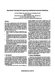
In BOP, multiple PPR instances are executed at the same time. A PPR is labeled by matching markers: BeginPPR(p) and EndPPR(p). Figures 1 and 2 show the marking of possible loop parallelism and possible function parallelism respectively. Figure 3 illustrates the run-time setup. Part (a) shows the sequential execution of three PPR instances, P , Q, and R. Part (b) shows the speculative execution. The execution starts as the lead process. When the lead process reaches the start marker of P , mbP , it forks the first speculative process, spec 1, and then continues to execute the first PPR instance. Spec 1 jumps to the end marker of P and executes from there. When spec 1 reaches the start of Q, mbQ , it forks the

... BeginPPR(1); work(x); EndPPR(1); ... BeginPPR(2); work(y); EndPPR(2); ...

... while (1) { get work(); ... BeginPPR(1); work(); EndPPR(1); ... }

Figure 2. possible function parallelism

Figure 1. possible loop parallelism

lead process

( e me mQ R

(

R

(a) Sequential execution of PPR instances P, Q, and R and their start and end markers.

R (partial)

( R

(

(

spec 1 commits

spec 2 starts

e mQ

mRb

Q

Q

(

(

mRe

(

( (

mRb

b mQ

(

e mQ

mPe

(

Q

(

Q

(

mb

P mPe understudy branch starts

spec 1 starts

(

P mPe

(

mPb

(

mPb

spec 2 finishes first and aborts understudy (parallel exe. wins)

spec 2 commits next lead

(b) A successful parallel execution, with lead on the left, spec 1 and 2 on the right. Speculation starts by jumping from the start to the end marker. It commits when reaching another end marker.

Figure 3. An illustration of the sequential and the speculative execution of three PPR instances

second speculative process, spec 2, which jumps ahead to execute from the end of Q. At the end of P , the lead process starts an understudy process, which reexecutes the following code nonspeculatively. The lead process itself then waits for spec 1 to finish, checks for conflicts; if no conflict is detected, it commits its changes to spec 1, which assumes the role of the lead process so later speculation processes are handled recursively in a similar manner. The kth spec is checked and combined after the first k − 1 spec processes commit. BOP employs a set of techniques to efficiently detect conflicts for execution correctness [3]. One of the important features of BOP is that the understudy and the speculative processes execute the same PPR instances. The understudy’s execution is part of a sequen-

tial execution of the program and thus is absolutely correct; on the other hand, the speculative execution starts earlier but contains more overhead and is subject to possible dependence violations. They form a sequential-parallel race. If the speculation completes earlier correctly, the parallel run wins and the parallelism is successfully exploited; otherwise, the understudy’s run guarantees the basic efficiency of the program. In the latter case, the speculative processes abort, and their execution becomes a waste of computing resource.

3

Adaptive Speculation

To avoid the waste caused by failed speculative executions, we develop a statistical predictor that learns from prior instances of a PPR and predicts the profitability of its future instances. The output of the predictor is a binary value, indicating whether a PPR instance is profitable to be speculatively executed. This prediction task resembles branch prediction, but differs in two aspects. First, in branch prediction, the correctness of a prediction can always be determined immediately after the branch is resolved, whereas, in adaptive speculation, the profitability of a PPR instance cannot be uncovered unless the instance is speculatively executed. So, if a PPR instance is predicted as not beneficial and is not speculatively executed, the correctness of the prediction will remain unknown. The adaptive speculation, therefore, has to learn from the partial information. The second difference is that branch prediction is usually implemented on hardware with strict constraints on both space and time, whereas, adaptive speculation is a software scheme, permitting more sophisticated algorithms. The adaptive algorithm to be presented focuses on loop parallelism; it learns from prior iterations of a loop PPR. For the purpose of clarity, the following description assumes the speculative depth to be 1—that is, there is at most one speculation process at any time. Figure 4 shows the adaptive algorithm. In this algorithm, the array element gain[i] records the exponentially decayed average of the speculation success rate of P P Ri . The decay factor is γ (0 ≤ γ ≤ 1); the higher it is, the faster the influence of a past speculation decays. The element quota[i] records the number of the instances of P P Ri that have been executed without speculation since the previous failed speculation. The factor β is the aggressiveness factor; the higher it is, the less quota is needed for resuming the speculative execution. The gain threshold, G TH (0 ≤ G T H ≤ 1), determines the tolerance of the adaptive scheme to speculation failures; the higher it is, the more likely occasional failures of speculative execution will disable the speculation of the next several PPR instances.

(1)

gain[i] = 1; quota[i] = 0;

(2) run to BeginPPR(i)

gain[i] + quota[i] *β < G_TH?

Y

quota[i] = 0; execute with speculation

(3) Figure 5. Basic patterns of speculation profitability. (|: profitable; ¦: non-profitable.)

N speculation succeeds?

N

4

Y g=1

quota[i] ++; execute without speculation

Evaluation

g=0

gain[i] = γ *g + (1- γ )*gain[i]

This section first presents the accuracy of profitability prediction of the adaptive algorithm, and then reports the improvement of the computation efficiency of BOP system.

4.1

Prediction Accuracy

Figure 4. Adaptive algorithm

In the algorithm, both a successful speculation and a non-speculative execution (also called a skipped speculation) of a PPR instance contribute to the sum that triggers the next speculation (the white diamond box in Figure 4). The contribution from a successful speculation ranges from γ ∗ (1 − G T H) to γ, and a skipped speculation contributes β. Intuitively, a non-speculative execution should not be more encouraging than a successful speculation. Therefore, β should usually be smaller than γ ∗ (1 − G T H) (and greater than 0). The adaptive algorithm has three important features. First, the number of consecutive skips is limited by a constant upperbound, G T H/β. This property prevents BOP from skipping a whole parallelizable phase that follows a long unprofitable phase (i.e., pattern 2 followed by pattern 1 in Figure 5). Second, the algorithm learns from not only recent failures but also long-term speculation success rate. This property is useful for the algorithm to tolerate occasional abnormal events. Meanwhile, the use of decay helps the algorithm respond quickly to phase changes. The third property is that the aggressiveness in trying a speculation is a tunable factor (β) separated from the tolerance to speculation failures (G T H), enabling more flexible control. In the integration of the algorithm into BOP, the lead process conducts all the operations of the algorithm except those in the grey boxes in Figure 4. The answer to the question in the grey diamond box comes from the winner of the race between the understudy and the spec process. The new lead process (i.e., the winner of the race) conducts the operations in the two grey rectangle boxes.

To comprehensively evaluate the adaptive schemes, we test the algorithm on a series of profitability patterns. The three basic patterns are showed in Figure 5. The first pattern is when unprofitable speculations are rare; the second is when the profitable speculations are rare; the third is when unprofitable and profitable speculations are evenly mixed. The pure randomness of the third pattern determines that no algorithms can predict the instances in the pattern with an accuracy consistently higher than 50%. Therefore, we focus on the first and the second patterns. In addition, we use their combined patterns to test the capability of the adaptive algorithm in handling pattern changes. A combined pattern consists of a number of equal-length subsequences of the two basic patterns that interleave with each other. For each (basic or combined) pattern, we create a biased random sequence composed of 200,000 elements. An element is either 0 or 1, respectively standing for PPR instances that are profitable or unprofitable to be executed speculatively. The two basic patterns respectively contain 10% and 90% dependences. We use 4 combined patterns; the length of a subsequence in them is respectively 10, 100, 1000, and 10000. The prediction accuracy is defined as follows: accuracy =

|Spec ∩ P rof | + |Spec ∩ P rof | , |P rof ∪ P rof |

where, Spec is the set of PPR instances that are executed speculatively, and Prof is the set of PPR instances that are profitable to be speculated. Thus, the denominator in the criterion is the total number of opportunities for (successful and non-successful) speculation, which is equal to half the total number of PPR instances; the numerator is the number of correct predictions for both profitable and non-profitable PPR instances.

100

80

80

80

60 40 20

Accuracy (%)

100

Accuracy (%)

Accuracy (%)

100

60 40

0.2

0.4

γ

0.6

0.8

1

0 0

40 20

20

0 0

60

0.2

(a) Decay factor

0.4 0.6 G_TH

0.8

1

(b) Gain threshold

0 −3 10

−2

10

−1

β

10

0

10

(c) Aggressiveness factor

Figure 8. The effect of each individual parameter in the adaptive algorithm. The seminal configuration is as follows: γ = 0.4, G T H = 0.25, β = 0.0073.

Table 1. Profitability prediction accuracy∗ 90

Patterns 1 2 (1,2)-102 (1,2)-103 (1,2)-104 (1,2)-105

Accuracy (%)

80

70

60

accl − accg (%) 0.6 3.2 1.5 0.2 1.0 1.8

(γ, G T H, β)l (0.25, 0.3, 0.0159) (0.05, 0.9, 0.0001) (0.85, 0.1, 0.0084) (0.35, 0.25, 0.0085) (0.2, 0.25, 0.0021) (0.05, 0.65, 0.0002)

∗ accg is the accuracy using the globally-chosen configuration; accl is for the locally-chosen configuration; (γ, G T H, β)l shows the corresponding configurations.

50 0

accg (%) 89.6 86.8 77.2 86.2 88.0 88.2

500 1000 1500 2000 2500 3000 3500 Configurations

Figure 6. Prediction accuracies using different configurations. The configurations in a panel (i.e., the area between two adjacent vertical lines) have the same value of γ. The order of the configurations follows the loops in Figure 7.

for (γ=0.05; γ < 1; γ+=0.05){ for (G TH = 0.05; G TH