ABSTRACT. We present an adaptive spectral technique for ground clutter and noise suppression in weather radar echoes. This technique is especially good for ...
ADAPTIVE TECHNIQUE FOR CLUTTER AND NOISE SUPRESSION IN WEATHER RADAR EXPOSES WEAK ECHOES OVER AN URBAN AREA Svetlana Bachmann 1, 2, 3, Victor DeBrunner 4, Dusan Zrnic 3, Mark Yeary 2 1
Cooperative Institute for Mesoscale Meteorological Studies, 2 The University of Oklahoma 3 National Severe Storm Laboratory, NOAA/OAR 4 Florida State University ABSTRACT
We present an adaptive spectral technique for ground clutter and noise suppression in weather radar echoes. This technique is especially good for detecting weak echoes that are either submerged in noise or masked by the residuals from ground clutter if standard techniques for clutter suppression are used. Our technique is demonstrated on two clear air cases observed with Doppler weather radar on February 22, 2007 and March 6, 2007. Adaptively suppressed ground clutter and noise allow exposure of a feature over an urban area, which we interpret as a “bird highway” between two lakes and along the river. Index Terms— frequency domain analysis, radar terrain factor, clutter, noise measurement, adaptive signal processing. 1. INTRODUCTION Any weather radar data from low elevation angles is affected by returns from motionless ground clutter (GC). Ground clutter can be suppressed using different techniques. Among these the best performances are achieved by the frequency domain filters (i.e., an adaptive notch and Gaussian model adaptive processing) [1]-[5]. Frequency domain processing is geared toward examining echoes by the shape of their power spectral density. Generally, the frequencies are converted to corresponding Doppler velocities in the unambiguous interval (from –va to va). The contribution from ground clutter, in this representation, is a peak located at zero Doppler velocity. The contribution from a group of moving/blown scatterers is a peak located at the mean radial velocity of the scatterers (assuming absence of velocity ambiguities or folding). Often echoes in one resolution volume are caused by both ground clutter and moving scatterers. Therefore, when the ground clutter spectral coefficients are removed, the remaining spectral coefficients can be summed to estimate the power of the filtered echo. Some filters interpolate the gap left from the removed spectral coefficients. GMAP fits a Gaussian curve to fill in the gap [4], [5]. Interpolation and Gaussian fit
might mistakenly add power to the observed signal. The added power is negligible in the conditions of high signal to noise ratio (SNR), and is unacceptable in the conditions of low SNR. An adaptive notch leaves the gap open, does not add power, and therefore, performs well in any SNR condition. In such manner the ground clutter echoes are suppressed and the echoes from moving scatterers are unveiled. However, the unveiling of echoes hidden by ground clutter does not occur when the signal of interest is weak or has a narrow spectral spread. Up to this time such signals are lost below noise threshold and are not considered reliable [2], [6], [7]. Some current radar applications can benefit from detecting weak signals. Among these are wind profiling in clear air conditions, the study of reflectivity plumes, refractivity retrieval, and the surveillance of bird and insect movements [6], [8]-[12]. Furthermore, an ongoing upgrade of weather surveillance radars (WSR-88D in the National Weather Service’s network) to dual polarization requires splitting transmitted power onto two channels, leading to a loss in sensitivity of 3 dB. The radar is capable of detecting weak signals even if the background clutter power surpasses signal power [2], [11]. Yet, the existing techniques do not utilize this capability [6]. We present a spectral technique in which an adaptive notch on the ground clutter coefficients is performed after the power spectral density is adjusted relative to the inherent spectral noise level. In current radar applications noise is considered to be a single value that is applied to the entire 360° azimuthal range of a given elevation. We show that the level of spectral noise changes drastically at the regions with airborne and ground clutter. This change often can be attributed to the rise of spectral skirts due to modulations and/or saturation. The level of spectral noise at other regions does not significantly change and accurately represents radar system noise. Our technique reveals that echoes currently considered to have low signal to noise ratios may actually have sufficient “spectral peak power” to “noise level” ratio. Like all frequency domain filters, our technique requires a sufficient number of pulses (samples) for spectral processing [2], [7]. We demonstrate this technique using time-series data collected in clear air conditions and with
settings of a current operational batch mode [6]. We show that 41 samples of the batch mode are sufficient for spectral analyses. Our technique allows us to suppress clutter from the Oklahoma City Metro area and to expose weak reflectivity plumes, echoes from birds, and an unexpected feature above the urban area. This feature is a track with higher than background reflectivity values that appear to connect two lakes around the city. We attribute this track to birds. We re-examined the revealed echoes with a finer spectral resolution (128 samples verses 41 sample of the batch mode) and in the dual polarization mode. Dual polarization allows evaluation of geometric properties of the detected scatterers [2], [9], [11], [12]. We present a map of the spectral noise level and compare it to the map of ground clutter. The maps of spectral noise levels from two sets of data and from two polarizations are similar, but not identical, and are subjects for further investigation.
3. 4. 5.
6.
The noise level is estimated as a mean value of the lower half of the ordered spectral coefficients. The power is adjusted relative to the noise level (PSD is shifted such that noise in all range locations is at the same level). The power in the spectral coefficients at and near zero velocity is compared to the noise level. The depth to which spectral coefficients are subjected to comparison is determined by the number of pulses used and the expected spectral width of GC. In the presented examples, the total number of spectral coefficients which could be considered as GC does not exceed 7 for 41 samples, and does not exceed 12 for 128 samples. These adjustable figures are determined experimentally. The ground clutter coefficients are notched. The remaining spectral coefficients use used for power computation.
2. RADAR SET UP AND DATA COLLECTION
4. EXAMPLES OF CLUTTER SUPRESSION
Time-series data were collected with the research S-band Doppler polarimetric radar (KOUN) that is maintained and operated by the National Oceanic and Atmospheric Administration/National Severe Storm Laboratory (NOAA/NSSL) in Norman, OK. Two sets of data are collected in clear air conditions and at elevation 0.5° on February 22, 2007 at 3 pm (20 UTC) and on March 6, 2007 at 3 pm (20 UTC). On February 22, 2007 the radar was in the single polarization mode, imitating the operational batch mode. The batch mode technique uses alternating long and short pulse repetition time (PRT) on each radial for one full 360° rotation [6]. A long PRT of 3106 μs and 4 pulses is sufficient to obtain intensity and location information. A short PRT of 986 μs and 41 pulses allows for more accurate velocity estimation. The batch mode uses a DC removal on the long PRT to suppress ground clutter. We used 41 pulses of the short PRT for adaptive spectral filtering, because 4 pulses of long PRT are not sufficient for spectral analyses. Optically clear air and a light S-SE wind were reported on the day of the experiment in February. On March 6, 2007, the radar was in dual polarization mode and scanned 360° with a PRT of 780 μs and 128 pulses for spectral processing. Clear air and a light S-SW wind were reported on the day of the experiment in March.
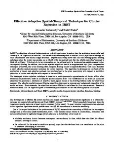
Fig. 1 shows the reflectivity Z of clear air for February 22 and March 6 in the left and right columns respectively. The radar is in the center of each image; the range extends outwards and is shown only to 50 km to exemplify ground clutter returns. The reflectivity in Figs. 1a, 1b contain ground clutter returns and expose echoes caused by the structures of the Oklahoma City urban area and the shape of the terrain. In Figs. 1c, 1d the ground clutter returns are removed with an adaptive notch filter. However, the ground clutter residuals are still visible. Figs. 1e, 1f show reflectivity obtained using our technique. The ground clutter coefficients are notched after the spectral noise level was adjusted. The notch parameters are the same as in Figs. 1c, 1d. The weak echoes from clear air and the echoes from foraging birds become apparent.
3. TECHNIQUE The technique is performed on time-series data in the frequency domain. For each range location the following steps are performed: 1. Fourier analysis is used to obtain the power spectral density (PSD) from the echo voltage multiplied by a window function (we use the Blackman window [2]). 2. Spectral coefficients are sorted in ascending order of their powers.
4.1 Comparing reflectivity with/without clutter filters The scatter plots of reflectivity are depicted in Fig. 2. Range locations from 0 to 30 km, where ground clutter dominates, are used for these analyses. The scatter plots are color coded to distinguish regions with different scatter densities. The reflectivity for February 22 and March 6 are shown in left and right columns respectively. Figs. 2a, 2b show scatter plots of unfiltered reflectivity Zo and reflectivity after ground clutter was removed with an adaptive notch filter Zf. The Zo of 60 dB is suppressed to about 20 dB level, and Zo of 40 dB is suppressed to about -10 dB on both days. Figs. 2a, 2b depict suppression levels reaching 50 dB. Figs. 2c, 2d show scatter plots of unfiltered reflectivity Zo and reflectivity after the GC was removed with an adaptive notch with adjusted spectral noise level, Zfn. There are regions on these plots that indicate the clutter suppression level 80 dB. Fig. 2c compares Zf and Zfn.
March 6, 2007, 3 pm, el. 0.5°
February 22, 2007, 3 pm, el. 0.5° 80
Z (dB)
Zf (dB)
Range (km)
Range (km)
80
(a)
(b) 40
40
60
20
40
0
20
20
0
Range (km) March 6, 2007, 3 pm, el. 0.5°
(c)
Z (dB)
20 40 Zo (dB)
60
-20 -20
80
February 22, 2007, 3 pm, el. 0.5°
(d)
60
20 40 Zo (dB)
60
80
0
(d)
40
20
Zfn (dB)
Zfn (dB)
Range (km)
0
March 6, 2007, 3 pm, el. 0.5°
(c)
60 40
Range (km)
100 80
-20 -20
February 22, 2007, 3 pm, el. 0.5°
Occurrence
60
0
Range (km)
March 6, 2007, 3 pm, el. 0.5°
(b)
60
Zf (dB)
February 22, 2007, 3 pm, el. 0.5°
(a)
0 -20
20 0 -20
-40 -40
-60
Range (km) March 6, 2007, 3 pm, el. 0.5°
(e)
(f)
-40
50
February 22, 2007, 3 pm, el. 0.5° 40
Z (dB)
60
(e)
40
20
Zfn (dB)
0 -20
0 20 Zo (dB)
40
60
March 6, 2007, 3 pm, el. 0.5°
(f)
0 -20
-40 -60 -60
Range (km)
-20
20
Range (km)
Range (km)
February 22, 2007, 3 pm, el. 0.5°
0 Zo (dB)
Zfn (dB)
Range (km)
-50
Range (km)
Fig. 1. Examples of clutter suppression: (a, b) unfiltered reflectivity, (c), (d) reflectivity filtered using the adaptive notch, (e, f) reflectivity filtered using the same adaptive notch but with adjusted level of spectral noise. The data from February 22 (left column) and March 6 (right column) have 41 and 128 samples for spectral analyses respectively. Echoes within 50 km range are displayed to expose the returns from ground clutter.
A large region with small reflectivity values between -10 dB and 20 dB that is not suppressed by the notch filter alone is the ground clutter residuals (Figs. 1c, 1d). Adjustment of spectral noise level successfully removes these residuals (Figs. 1e, 1f) and reveals the weak echoes. 4.2 Importance of the correct noise value Our technique shows that the spectral noise level changes rapidly especially at ranges close to the radar and cannot be represented by a single value, as is generally assumed. It was known that the level of spectral noise affects performance of the ground clutter filter. For example, the Gaussian model adaptive processing (GMAP) is a spectral ground clutter filter that fits a Gaussian curve instead of simple notching the spectral coefficients that are suspect to be ground clutter [4], [5]. The GMAP has an option to determine the noise level from spectra or to use the provided
-40 -60
-40
-20 0 Zf (dB)
20
40
-50
0 Zf (dB)
50
Fig. 2. Reflectivity scatter plots: (a, b) unfiltered reflectivity Zo vs. reflectivity filtered using the adaptive notch Zf, (c, d) Zo vs. reflectivity filtered using the adaptive notch with adjusted level of spectral noise Zfn, (e, f) Zf, vs. Zfn. The data are from February 22 (left column) and March 6 (right column). Echoes within 30 km range are used for these analyses.
noise. We used GMAP with our data to illustrate how the performance of the filter changes when the correct noise is used. Fig. 3a shows scatter plot of power unfiltered verses filtered using the GMAP with the noise value provided by the system. Fig. 3b shows scatter plot of power unfiltered verses filtered using GMAP with the adaptive noise determined from spectra. Fig. 3c compares the powers filtered using GMAP with provided and estimated noises. In this example of clear air, the performance of filter with adaptive noise is improved for the signals with small powers; large powers are not greatly affected. Insignificant powers of small ground clutter or its residuals are still a significant inconvenience because when not filtered such returns would bias velocity estimate toward zero. In clear air condition these insignificant powers become dominant and mask the weak signals from clear air. This motivated us to create a map of level of spectral noise, to investigate its features, and to compare it to the map of ground clutter.
g
4.4 “Bird highway” The reflectivity (Figs. 1e, 1f) depicts smooth area with echoes from clear air and point echoes from birds. Birds are more numerous in the data from March compared to data from February. A similar feature is visible in both reflectivity images. The feature is at about 20 km north from the radar (Figs. 1e, 1f) and does not coincide with major roads on the ground. It exposes a path through Oklahoma City and Metro area. Fig. 5 displays the zoom to this feature superimposed on a map of lakes. Spectral analyses of this feature indicate that there are contributions from strong point scatterers as well as a contribution from weak distributed scatterers. The point scatterers are moving at different velocities and have narrow peaks in spectrum that
40 20 0
40
Performance of GMAP with determined noise
20
-20
0 -20 -40
-40 -60 -60
-40
-20 0 So (dB) 40
SGMAPan (dB)
20
20
-60 -60
40
(c)
-40
-20 0 So (dB) 100
60
-20
40
-40
20
-40
40
80
0
-60 -60
20
-20 0 SGMAP (dB)
20
40
Occurrence
S GMAP (dB)
(b)
Performance of GMAP with provided noise
S GMAPan (dB)
(a)
0
Fig. 3. Scatter plots of power with/without GMAP: (a) unfiltered power So vs. power filtered with GMAP with provided noise SGMAP, (b) So vs. power filtered with GMAP with determined adaptive noise SFMAPan, (c) SGMAP, vs. SGMAPan. The data from February 22 have 41 samples for spectral analyses. Only ranges between 0 and 30 km are used for these analyses. March 6, 2007, 3 pm, el. 0.5°
(a)
(b)
Power (dB)
Range (km)
Range (km)
February 22, 2007, 3 pm, el. 0.5°
Clutter map°
Clutter map°
Range (km)
Range (km)
February 22, 2007, 3 pm, el. 0.5°
March 6, 2007, 3 pm, el. 0.5°
(c)
(d)
Power (dB)
Range (km)
Range (km)
4.3 Maps of clutter and noise The ground clutter maps (Figs. 4a, 4b) are obtained by averaging power from three spectral coefficients near zero velocity. The “noise” is obtained as described in Section 3. We use quotes for “noise” in the figures to emphasize that the level of spectral skirts can be different from the radar system noise. There are similarities between the maps of ground clutter and the maps of spectral noise. Both maps reflect the shape of ground clutter, although the powers are significantly different. There are differences in the maps of spectral noise for different data sets (Figs. 4c, 4d). Though the noise level map is closely related to the ground clutter map, it also depicts or enhances other features and artifacts. For example, echoes from structures near the radar include the moving traffic on Interstate I-35. These echoes appear as a distinct line located about 2 km west from the radar and stretching North to about 20 km range ring. The echoes from I-35 are well pronounced. These echoes are similar to echoes from tornado debris by having extremely wide spectral spread. Ground vehicles moving with different speeds produce multiple peaks in main and side lobes of the radar beam. The echoes are strong and superimposed on each other. This raises the level of estimated spectral noise. In such situations, the detection of a weak atmospheric echo is extremely difficult, and is possible only if the spectra in resolution volumes adjacent to the ones with road have sufficient strength (power and spectral width) for the peak produced by atmospheric echo. Another road is visible at about 17 km north from the radar. This road is interstate I240 that in fact stretches East-West, but appears as a bend curve due to geometry of the radar scan. Many point echoes in the noise map are from airplanes. Therefore a possible application of spectral noise map is the aircraft detection and tracking. The maps of spectral noise level in two polarizations (not shown) do not exactly match. The noise maps in Figs.4c, 4d indicate the level of noise at further ranges (that is expected to represent the radar system noise) is different for the two days of observation. It is -78 dB in February and -90 dB in March due to different sampling.
“Noise” map° Range (km)
“Noise” map° Range (km)
Fig. 4. Power PPIs (a, b) ground clutter, (c, d) the level of spectral noise. The data from February 22 have 41 samples for spectral analyses. We use quotes for “noise” in the figures to emphasize that the level of spectral skirts can be different from the radar system noise.
are spaced around a wider and smaller wind peak with about 10 m s–1 difference (Fig. 5) in both directions. The weak spectral peak caused by wind is recognized by continuity of spectral peaks in range and in agreement with atmospheric sounding. Comparing the terrain map with the reflectivity map we observed that the feature north of the radar appears to connect two lakes in the Oklahoma City vicinity, Lake
Lake Hefner
both sides of the wind path indicating that birds travel in both directions. The values of the polarimetric spectral densities are not calibrated.
North Canadian River 0°
330
30°
6. CONCLUSION Adaptively computing spectral noise levels allows one to expose weak echoes veiled by ground clutter residuals. Replacing the single value for noise by the adaptive noise level allows us to improve the GC suppression and to utilize the echoes that are currently considered to have low signal to noise ratios but may actually have sufficient “spectral peak power” to “noise level” ratios. 7. REFERENCES Range (km) Stanley Draper Lake
Fig. 5. A map of lakes and rivers in the Oklahoma city metro area superposed on the feature exposed in Fig. 1c at about 20 km North from the radar (February 22, 2007 at 3 pm). Sh (dB)
(a)
30
-10
25
0
20
10
15 10
20
5
30 25
30
35
40
45
10
-10 0
5
10
0
20
-5
30 20
50
Range (km)
15
-20
25
30
35
40
45
φDP (deg.)
ρh
(c)
-30
0.95
)
-20
0.9
-10 0
0.85
10
0.8
20
50
Range (km)
Wind
(d)
150
-20
100
-10
50
–1
20
Birds
Velocity (m s–1 )
Velocity (m s–1 )
-20
-30
ZDR (dB)
(b)
-30
35
Velocity (m s
Velocity (m s–1 )
-30
0
0
10
-50
20
-100
0.75
20
-150
30
30 25
30
35
40
Range (km)
45
50
20
25
30
35
40
45
50
Range (km)
Fig. 6. Polarimetric spectral densities in a radial at 344° azimuth: (a) ShSD, (b) ZDRSD, (c) ρhvSD, and (d) φDPSD (March 6, 2007, 3 pm, el. 0.5°). Only powers above noise level and ρhv>0.7 are shown.
Hefner and Stanley Draper Lake. The path appears to curve south around the Oklahoma City downtown. Another broken path at about 355° azimuth and 35 km (Fig. 1g) is near Lake Overholser. We attribute non-wind spectral peaks to birds. Apparently, birds have a designated “highway” over the city connecting these two lakes in the vicinity. This is the first documentation of bird echoes unveiled from strong ground clutter background. Polarimetric spectral densities (of power Sh, differential reflectivity ZDR, copolar correlation coefficient ρhv and differential phase φDP) in a radial at azimuth 344° for the high spectral resolution data (March) are shown in Fig. 6. Polarimetric spectral densities expose a path from wind and multiple blobs from birds. Blobs are on
[1] J. Golden, “Clutter mitigation in weather radar systems filter design & analysis,” System Theory, SSST '05. Proc. 37th Southeastern Symposium on, pp. 386 – 390, 2005. [2] R. J. Doviak and D. S. Zrnic, Doppler Radar and Weather Observations, Academic Press, 1985. [3] G. Galati, Advanced Radar Techniques and Systems, Peter Peregrines Ltd., 1993. [4] A. D. Siggia, and R. E. Passarelli, Jr., “Gaussian model adaptive processing (GMAP) for improved ground clutter cancellation and moment calculation,” Proc., European radar conf., 67-73, 2004. [5] R. L. Ice, R.D. Rhoton, D. S. Saxion, C.A. Ray, N. K. Patel, D. A. Warde, A. D. Free, O.E. Boydstun, D. S. Berkowitz, J. N. Chrisman, J. C. Hubbert, C. Kessinger, M. Dixon, S. Torres, “Optimizing clutter filtering in the WSR-88D, ” AMS Proc. 23d Conf on IIPS, P2.11, 2007. [6] U.S. Department of Commerce/NOAA, Federal meteorological handbook #11: Doppler radar meteorological observations. Part C. WSR-88D products and algorithms, FCM-H11C-2006. [7] M. H. Hayes, Statistical Digital Signal Processing and Modeling. John Wiley & Sons, 1996. [8] G. L. Achtemeier, “The use of insects as tracers for clear air boundary-layer studies by Doppler radar,” J. Atmos. Oceanic Technol., 8, 746–765, 1991. [9] S. Bachmann, and D. Zrnic, “Spectral density of polarimetric variables separates biological scatterers in the VAD display,” J. Atmos. Oceanic Tech., Amer. Meteor. Soc., in print, 2007. [10] T. J. Lung, S. A. Rutledge, and J. Smith, “Observation of clear air Dumbbell-shaped echo patterns with the CSUCHILL polarimetric radar,” J. Atmos. Ocean. Technol., 21, 1182-1189, 2004. [11] D. Zrnić, and A. Ryzhkov, “Observation of Insects and Birds with Polarimetric Radar,” IEEE Trans. Geosci. Remote Sens., 36, 661-668, 1998. [12] T. Schuur., A. Ryzhkov, P. Heinselman, D. Zrnic, D. Burgess, and K. Scharfenberg, “Observations and classification of echoes with the polarimetric WSR-88D radar,” NSSL report, October, NOAA/OAR, Norman OK, 2003.