SPIE Proceedings: Signal and Data Processing of Small Targets, Vol. 4048, Orlando, FL, 2000.
Effective Adaptive Spatial-Temporal Technique for Clutter Rejection in IRST Alexander Tartakovskya and Rudolf Blaˇzekb a Center
for Applied Mathematical Sciences, University of Southern California 1042 West 36th Place, DRB-155, Los Angeles, CA 90089-1113, USA b Department
of Mathematics, University of Southern California 1042 West 36th Place, DRB-155, Los Angeles, CA 90089-1113, USA ABSTRACT In IRST applications, cluttered backgrounds are typically much more intensive than the equivalent sensor noise and intensity of the targets to be detected. This necessitates the development of efficient clutter rejection technology for track initialization and reliable target detection. Experimental study shows that the best existing spatial filtering techniques allow for clutter suppression up to 10 dB, while the desired level (for the reliable detection/tracking) is 25-30 dB or higher. This level of clutter suppression can be achieved only by implementing spatial-temporal rather than spatial filtering. In addition, the clutter rejection algorithm should be supplemented by a jitter compensation technique. Otherwise, due to the blurring effect, temporal filtering cannot be applied effectively. This paper discusses a novel adaptive spatial-temporal technique for clutter rejection. The algorithm is developed on the basis of the application of robust and adaptive methods that are invariant to the prior uncertainty with respect to statistical properties of clutter and adaptive with respect to its variability. The developed clutter rejection technique is based on a multi-parametric approximation of clutter which, after estimation of parameters, leads to an adaptive spatial-temporal filter. The ‘coefficients’ of the filter are calculated adaptively to guarantee a minimum of empirical mean-square values of the filtering residual noise for every time moment. The adaptive spatial-temporal filtering algorithm allows one to suppress any background, regardless of its spatial variation. Simultaneously, the algorithm estimates LOS drift and allows for jitter compensation. Results of simulation show that the algorithm gives a tremendous gain compared to the best existing spatial techniques. Keywords: Infrared Search and Track (IRST), adaptive spatial-temporal clutter rejection, detection, tracking.
1. INTRODUCTION The development of efficient IR clutter rejection and target preservation/enhancement algorithms is of critical importance for modern Infrared Search and Track (IRST) systems.1–4,9,10,12,16 This is especially important, since the targets are usually weak and of small spatial extension (a few pixels). To meet technical requirements the advanced clutter rejection algorithms should provide more than 30 dB improvement in detection sensitivity. One of the major limitations of the performance of IR/EO sensors is the uncertainty of LOS and its non-regular changes due to vibrations (LOS stabilization jitter). This nuisance factor results in translational, rotational, and parallax distortions in registered images (jitter-noise due to instability). Jitter leads to: • relatively stationary clutter becomes non-regular, non-stationary in time, which does not allow for efficient temporal filtering of clutter; • the estimated (in the sensor’s coordinate system) target location deviates from true coordinates by the value of unknown and varying in time shift. Send correspondence to Alexander Tartakovsky: Email:
[email protected]; Telephone: 213-740-2450; Fax: 213-740-2424; WWW: http://www.usc.edu/dept/LAS/CAMS/usr/facmemb/tartakov
1
Existing methods of sensor stabilization (mechanical/electronical) are very expensive and are not efficient enough. Perhaps this is one of the major reasons why current IR scanning and staring array sensors employ primarily spatial, rather than spatio-temporal, processing to accomplish clutter rejection.1,10 In this work, we propose the following idea, which allows us to avoid the use of expensive equipment for “superstabilization”. The exterior clutter is itself the source of valuable information about current position of the sensor’s coordinate system. Indeed, clutter typically changes slowly (highly correlated) during certain periods of time which allows us to consider it as almost constant during these intervals. Thus, any temporal changes in these intervals occur only due to jitter. Since clutter is normally much more intensive than sensor noise, there is no problem of high ‘SNR’ for compensation (which is a real problem for compensation based on reference signals from point sources). Once jitter is compensated, we can solve not only the problem of spatial filtering but, also, the problem of temporal filtering (i.e., spatial-temporal clutter rejection) efficiently. In this case, clutter can be suppressed to the level of sensor noise. Below, we develop a 3D spatial-temporal filtering technique for clutter rejection. This method includes a jitter estimation and compensation algorithm as a non-separable part. The proposed clutter rejection method does not use any assumptions on statistical models of clutter such as Gaussian field, which are highly unreliable and lead to non-robust algorithms. All we need for efficient temporal processing is the condition that clutter does not change substantially on certain time intervals. The developed clutter rejection technique is based on a multi-parametric approximation of clutter which, after estimation of parameters, leads to an adaptive nonlinear spatial-temporal filter. The ‘coefficients’ of the filter are calculated adaptively according to the maximum likelihood algorithm. The adaptive spatial-temporal filter allows one to suppress any background, regardless of its spatial variation. The 3D spatio-temporal filter not only whitens the data but also corrects all translational, rotational and parallax distortions. Results of simulation show that the algorithm gives a tremendous gain compared to the best existing spatial techniques. This paper is organized as follows. In Section 2, we formulate the problem and describe basic assumptions and constraints. Section 3 is a centerpiece. Here, we develop the two algorithms for clutter rejection and jitter compensation. The first one is based on the multi-parametric approximation of clutter by decomposing it as a sum of products of unknown parameters and given spatial basis functions. The Fourier basis or wavelet basis may serve as examples. In the algorithm, these parameters are estimated along with the jitter according to the maximum likelihood principle. Since the support of the basis and the number of terms in the sum are chosen in advance, we call this algorithm a ‘Fixed Support’ algorithm (‘FS-Algorithm’). The second algorithm is based on the spline approximation where not only the parameters of the approximation, but also the support of the approximation, are unknown. A simple example of such approximation is a step-wise constant approximation in unknown domains. In this case, not only the ‘amplitudes’, but also the domains, should be estimated. We call this algorithm an ‘Adaptive Support’ algorithm (‘AS-Algorithm’). Finally, in Section 4, we provide the results of simulations that allow one to evaluate the performance of the developed algorithms.
2. PROBLEM FORMULATION AND ASSUMPTIONS Assume an IRST system registers the sequence of 2D frames Y n = bn + ξ n ,
n = 1, 2, . . . ,
(2.1)
where Y n = {Yn (r ij ), i = 1, . . . , N1 , j = 1, . . . , N2 } is the frame of intensities, ξ n = {ξn (r ij ), i = 1, . . . , N1 , j = 1, . . . , N2 } is the sensor noise, bn = {bn (r ij + δn (r ij )), i = 1, . . . , N1 , j = 1, . . . , N2 } is clutter, and where δ n = {δn (r ij ), i = 1, . . . , N1 , j = 1, . . . , N2 } is the vector of unknown shifts that occur due to the jitter, r ij = (xi , yj ) is the pixel in the plane image with coordinates (xi , yj ). The following assumptions on noise, clutter, and jitter are used throughout the paper: 1. Noise in both time and space with Eξn (r) = 0 and Eξn (r)2 = σ 2 , where r = (x, y), ξn (r) is uncorrelated 2 i.e. ξn (r ij ) ∼ N (0, σ ), n = 1, 2, . . . , i = 1, . . . , N1 , j = 1, . . . , N2 are independent and identically distributed Gaussian random variables with mean zero and known variance σ 2 . 2
2. Clutter bn (r) is an arbitrary, unknown function of r and slowly-changing function of n in the following sense: there exists such interval T that
|bn+T (r) − bn (r)| ≤ σ
for all n and r.
(2.2)
3. Vibrations of the platform can be very fast such that the jitter δn (r ij ) can change abruptly from frame-to-frame, but these changes do not exceed some known value δmax (physical constraint). In the worst case scenario, we assume that the shift δn (r ij ) depends on the pixel r ij and may substantially change from pixel to pixel. This assumption allows us to take into account not only translations but, also, rotations and parallax. Parameter T defines the length of the interval in which clutter is a quasi-stationary process. This parameter is estimated experimentally and corresponds to the length of the temporal window where temporal filtering may be done. In other words, spatial-temporal filtering for clutter rejection is based on the data (Y n , . . . , Y n+T −1 ). To solve the clutter rejection problem, we must construct an estimate ˆbn (r) of the function bn (r) (on the basis of the data Y n−T +1 , . . . , Y n ) such that the difference ∆n (r) = bn (r) − ˆbn (r) would be small for all r. The reasonable practical requirement “would be small” is |∆n (r)| ≤ c · σ
for all r,
(2.3)
where c is a positive number (c = 1, say), while the values of the background bn (r) are usually much greater than the standard deviation of the noise σ. Note that in the model (2.1), for the sake of simplicity, we assumed that there is no signals from targets in frames. The idea of the approach to clutter suppression is considered for this simplified model. In real world applications, however, one has to include a signal component and to consider signal preservation/enchancement issues along with clutter rejection. This problem will be considered elsewhere. See, however, Section 4 for general discussion of the signal preservation problem.
3. ADAPTIVE SPATIAL-TEMPORAL REJECTION FILTER We start with an explanation of the idea of jitter compensation, assuming that the function bn (r) is known. Then, the only unknown in (2.1) is the shift δ that should be estimated. According to Assumption 3 in Section 2, it is supposed that vibrations can be quite fast such that the δn (r ij ) can change abruptly from one frame to another, but these changes do not exceed some known value δmax . First, we consider an extreme case where the shift δn (r ij ) may substantially change from pixel to pixel. Evidently, this is the most difficult case. This model allows one to handle not only translational effects but, also, rotations and parallax. In the reverse situation, δn does not depend on r ij (parallel shift). This latter case is relatively simple. The intermediate case occurs when δn changes from column to column but is constant within a column, i.e. δn (r ij ) = δn (i) for j = 1, . . . , N2 , where i is the identity of the i-th column. Since the distribution of ξn (r ij ) is Gaussian, the maximum likelihood (ML) estimate of jitter δˆn = δˆn (r ij ) in the n-th frame is the solution of the following minimization problem 2 δˆn (r ij ) = arg min (3.1) Yn (r ij ) − bn (r ij + δ) . |δ|≤δmax
Note that the optimization problem (3.1) is a nonlinear problem. If the estimate δˆn (r ij ) is quite accurate in the sense that |bn (r ij +δn (r ij ))−bn (r ij + δˆn (r ij ))| σ, then obviously, the residuals Yen (r ij ) = Yn (r ij ) − bn (r ij + δˆn (r ij )) ≈ ξn (r ij ) will be close to sensor noise, which means that clutter is rejected.
The alignment of frames according to the method (3.1) will be called the ML-alignment.
Since in actuality the function bn (r) is unknown, it should be estimated simultaneously with the jitter compensation. As was mentioned in the previous section, we do not use any assumptions on statistical properties of clutter. All we assume is that clutter is an arbitrary function of spatial coordinates (normally a quite sharp function) and a slowly changing function of time in a certain interval T (see (2.2)). We now develop the two algorithms that are based on parametric approximations of the function bn (r). The first approximation is based on a set of spatial basis functions (Fourier, wavelets, etc.) with a fixed support; the second one uses a spline approximation with an adaptive support. 3
3.1. Parametric Approximation With a Fixed Support Introduce the following time-space splitting approximation of clutter: bn (r) ≈
M X
θk (n)fk (r),
(3.2)
k=1
where θk (n) are unknown and slowly changing in the interval T functions, fk (r) are given functions chosen from the best fitting criterion. In the clutter rejection algorithm, the functions θk (n) = θk are replaced with unknown constants θk that should be estimated based on the data Yn−T +1 , . . . , Yn . Let θˆk (n) denote an estimate of θk (n) in the time window [n − T + 1, T ]. Then the corresponding estimate of the background at time n and the approximation error have the form: M M X X ˆbn (r) = θˆk (n)fk (r). θˆk (n)fk (r), ∆n (r) = bn (r) − (3.3) k=1
k=1
Note that, here, we consider the approximation-estimation in the reference system of coordinates, i.e. when the shift (jitter) δ = 0. Non-zero jitter leads to a shifted model bn (r) ≈
M X
θk (n)fk (r + δn (r))
k=1
with unknown shift δn (r) which generally depends on both space and time. The functions fk (r) and the number M should be chosen so that the error of approximation ∆n (r) would satisfy the condition (2.3). This requirement may necessitate the use of a very large number, M , in cases where clutter has fast spatial variations. In fact, M can be comparable or even exceed the number of pixels N = N1 × N2 , which is typically in the order of 105 − 106 . 3.1.1. The clutter rejection algorithm: FS-Algorithm We now describe the first rejection filter which we call the FS-Algorithm. The abbreviations RCS and CCS are used for the reference coordinate system and corrected coordinate system, respectively. • Initialization. This step can be performed in different manners, and one such scheme is discussed later on. Typically this step requires at least T observations. In other words, for a chosen set of functions {fk (r)}1≤k≤M , we should estimate the unknown parameters θ = (θ1 , . . . , θM ), jitter δn , n = 1, . . . , T and clutter bT (r ij ) based on the initial T observations. Thus, the result of the initialization stage are the estimates θˆk (T ),
ˆbT (r ij ) =
(δˆ1 (r ij ), . . . , δˆT (r ij )),
M X
θˆk (T )fk (r ij + δˆT (r ij )).
k=1
• Typical Step n, n > T .
(a) Jitter Estimation. The estimate ˆbn−1 (r ij ) obtained from the previous step is compared with the n-th frame (starting with n = T ), and the ML estimate of jitter δˆn is computed as the solution of the following nonlinear optimization problem !2 M X ˆ ˆ (3.4) δn (r ij ) = arg min Yn (r ij ) − θk (n − 1)fk (r ij + δ) . |δ|≤δmax
(b) Estimation of Parameters in CCS. Having the estimates δˆn−T +1 (r ij ), . . . , δˆn (r ij ), the estimates θˆk (n) are computed for the n-th frame from the minimization problem∗ !2 M n X X −→ {θˆk (n)}. Ys (r ij ) − θk fk (r ij + δˆs (r ij )) (3.5) min θ
∗
k=1
s=n−T +1
k=1
Note that the estimator (3.5) is no more than the ML Estimator or, more generally, the Mahalanobis Distance Estimator.
4
This recomputing in the corrected coordinate system is equivalent to a ‘statistical alignment’ of frames. (c) Clutter estimation in CCS. Using the estimates obtained from (3.4) and (3.5), compute the estimate of bn (r ij ) for all i and j in the corrected coordinate system, ˆbn (r ij ) =
M X
θˆk (n)fk (r ij + δˆn (r ij )).
(3.6)
k=1
(d) Clutter Rejection. Using the estimate (3.6), compute the residuals (filtered background)
and check the condition
The Initialization Scheme
Yen (r ij , δˆn (r ij )) = Yn (r ij ) − |Yen (r ij , δˆn (r ij ))| ≤ Cσ
M X
θˆk (n)fk (r ij + δˆn (r ij )),
k=1
with C = 2 (for example).
n = 1: Do nothing and put δˆ1 (r ij ) = 0. n = 2: δˆ2 (r ij ) = arg min
|δ| N . When this is the case, we can require only approximate orthogonality. 3. The form of approximation should provide the single-valued solution to the optimization problem (3.4) with a small number of iterations and low error. 5
A good choice from the point of view of the approximation error would be the 2D Fourier decomposition b(x, y) =
M2 M1 X X
θk1 ,k2 exp{ι(k1 ω1 x + k2 ω2 y)}
with ω1 = α
k1 =1 k2 =1
2π 2π , ω2 = α , Mi = αNi , ∆x ∆y
in which case fk (r) = fk1 ,k2 (x, y) = exp{ι(k1 ω1 x + k2 ω2 y)}. Here α ≥ 1 (typically 2 or 3); ∆x and ∆y are resolutions in x and y directions; θk1 ,k2 are unknown coefficients that should be estimated. However, this choice leads to a very high computational complexity. Another good choice would be wavelet descriptors, which are often used in signal and image analysis. The members of a wavelet basis are mutually orthogonal, rescaled and shifted versions of a single ‘mother’ wavelet which has very special properties.8,11 In our model, the main benefit of using a wavelet basis is that, as opposed to the Fourier basis, the functions forming a wavelet basis for L2 (R) (and similarly for L2 (R2 ) which is our case) have compact support. In general, they are very efficient when describing functions with many jumps, edges, and similar local and ‘sharp’ features with ‘bad frequency properties’. This is often the situation in the case of clutter bn (r). Figure 1 shows the Haar mother wavelet which represents the simplest example of a wavelet basis of L2 (R). In the case of Haar decomposition, the function fk (r) has the following form fk (r) = fk1 ,k2 (x) × fk3 ,k4 (y),
where fs,l (z) = 2−s/2 ϕ(2−l z − s), ϕ(z) = 1l{0≤z T .
b k (T ), Ω
cT , M
δˆT ,
ˆbT (r) =
cT M X
k=1
θˆk (T )1l{r∈Ω b k (T )−δT (r)} .
(a) Jitter Estimation. The estimate ˆbn−1 (r ij ) obtained from the previous step, starting with n = T + 1, is compared with the n-th frame, and the ML estimate of jitter δˆn is computed as the solution of the following nonlinear optimization problem 2 cn−1 M X θˆk (n − 1)1l{rij ∈Ω δˆn (r ij ) = arg min Yn (r ij ) − b k (n−1)−δ} . |δ|≤δmax
k=1
bn (b) Estimation of Parameters in CCS. Having the estimate of jitter δˆn (r ij ), the estimates θˆk (n), Ω cn are computed for the n-th frame according to the iterative algorithm described above (see (3.10) and and M 7
(3.11)). The only difference is that these estimates are computed in CCS rather than in RCS, i.e. after the alignment of frames. (c) Clutter estimation in CCS. Compute the estimate of bn (r ij ) in the corrected coordinate system ˆbn (r ij ) =
cn M X
k=1
θˆk (n)1l{rij ∈Ω b k (n)−δˆn (r ij )} .
(d) Clutter Rejection. Compute the residuals (filtered background)
and check the condition
Yen (r ij , δˆn (r ij )) = Yn (r ij ) −
cn M X
k=1
|Yen (r ij , δˆn (r ij ))| ≤ Cσ
θˆk (n)1l{rij ∈Ω b k (n)−δˆn (r ij )}
with C = 2 (say).
4. RESULTS OF SIMULATION We start this section with the discussion of the performance indices. Recall that we left the problem of signal preservation for our future research. Despite this fact, we will now discuss this problem briefly. Let Sn (r ij ) and Sen (r ij ) be the original signal from the target and the signal after clutter rejection, respectively. Introduce the following indices: P P 2 2 e2 i,j Sn (r ij )Sn (r ij ) i,j Sn (r ij ) . , I2 = P I1 = P P Sen2 (r ij ) S 2 (r ij ) · Sen2 (r ij ) i,j
i,j
n
i,j
From the point of view of correct signal recostruction/preservation, a good algorithm should provide both I1 and I2 close to 1. If this is the case, then a good algorithm, from the point of view of clutter rejection, should maximize the value of σ2 G = 10 log 2in , (4.1) σout
2 2 is the variance of the output frame Ye n . Indeed, if the signal where σin is the variance of the input frame Y n and σout is preserved, then the maximization of G is equivalent to the maximization of the relative Signal-to-Noise-Plus-Clutter Ratio SNCRin 10 log SNCRout
where SNCRin =
sP
2 ij Sn (r ij ) 2 σin
,
SNCRout =
sP
ij
Sen2 (r ij )
2 σout
.
Thus, we will use the index G defined in (4.1) as the measure of the quality of the clutter rejection: the bigger G, the better the algorithm. In simulations we used a subset H of the Haar wavelet basis to approximate the clutter function bn (r) (see (3.8)).
In the observations Y k , k = 1, 2, . . . , n, the two-dimensional parallel jitter {δ k = (δx,k , δy,k )} was modeled by pairs of independent random variables uniformly distributed over the set {0, ±1, . . . , ±δmax }. The observations Y 1 , . . . , Y n were generated by applying n independent replicas of the jitter to the coordinates of the function b, and then, subsequently adding white Gaussian noise (with mean 0 and variance σ 2 ) to each component of a discretized version of the function b(r + δ k ). The discretization was obtained by evaluating the function b(r + δ k ) at 32 × 32 equispaced points in R2 , which have been selected beforehand in the reference coordinate system. Figure 2 illustrates the performance of the developed rejection filter for a particular case. In Figure 2, the picture on the left-hand side shows a typical input (cluttered and noisy) frame with the noise variance σ 2 = 10, clutter dynamic range (CDR) 10 − 100, and jitter δ ∈ [−2, +2] pixels. The picture on the right side shows the result of clutter rejection (the residuals at the output of the filter) with temporal window size T = 20 frames. It can be seen 8
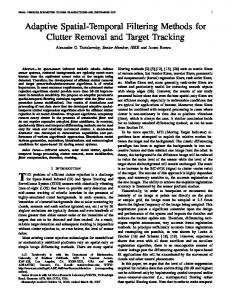
that clutter is completely removed and the residuals look like noise. For comparison, Figure 3 illustrates the result of spatial-only (in-frame) processing based on the nonparameteric method developed by Leonov.13 This spatial clutter rejection technique is based on nonparametric regression algorithms, namely, on kernel smoothing methods. This technique proved to be highly efficient for a variety of ‘difficult’ cluttered scenes, in particular for the IR LAPTEX field test data.13 In Figure 3, the picture on the left-hand side depicts the estimate of clutter, while the picture on the right-hand side shows the residuals at the output of the spatial filter. One can see that clutter is removed only partially. The pieces of residual clutter can be seen even by the naked eye. The advantage of the developed temporal-spatial filter over the spatial filter is obvious when comparing the right-hand side pictures in Figure 2 and Figure 3. The data in Table 4 summarize the performance of the rejection filter in terms of the gain G defined in (4.1), and also, in terms of other important characteristics: the values maxi,j Yn (r ij ) P dynamic range (maximum and minimum P and mini,j Yn (r ij )), mean value Y n = (N1 N2 )−1 i,j Yn (r ij ), and variance σY2 = (N1 N2 )−1 i,j [Yn (r ij ) − Y n ]2 . For the spatio-temporal filter, the residuals have zero mean value, the dynamic range is much less than in the input frame, and the variance is close to the variance of the noise (σY2 = 10.84 versus σ 2 = 10). These numbers show that clutter is suppressed down below the noise level. This allows us to arrive at the conclusion that the developed algorithm is highly efficient: it completely removes high-intensive clutter in the presence of substantially large jitter. Also, the data in Table 4 allow us to compare the nonparametric spatial filter with the developed spatial-temporal filter at the qualitative level. It can be seen that the dynamic range of the output frame of the spatio-temporal filter is 3 times smaller than that of the output frame of the spatial filter. The variance of the output frame of the spatio-temporal filter is over 10 times (10.3 dB) smaller than that of the output frame of the spatial filter.
30
30
25
25
20
20
15
15
10
10
5
5
0
0 0
5
10
15
20
25
30
0
5
10
15
20
25
30
Figure 2. Clutter Rejection: Spatial-Temporal Filter with the Haar Basis (σ 2 = 10, δ = ±2, CDR = 10 − 100, T = 20)
9
30
30
25
25
20
20
15
15
10
10
5
5
0
0 0
5
10
15
20
25
30
0
5
10
15
20
25
30
Figure 3. Clutter Rejection: Spatial Nonparametric Filter (σ 2 = 10, CDR = 10 − 100)
Table 1. Performance of Clutter Rejection Algorithms (σ 2 = 10, δ = ±2) Input Output (spatio-temporal), T = 20 Output (spatial)
Minimum 3.04 -10.24 -36.34
Maximum 105.25 9.44 34.60
Mean 56.10 -0.011 -0.004
Variance 482.86 10.84 114.99
Gain 16.5 (dB) 6.2 (dB)
5. DISCUSSION AND CONCLUSIONS The development of efficient IR clutter rejection algorithms is of critical importance for modern IRST systems. LOS stabilization jitter, which results in translational, rotational, and parallax distortions in registered images, does not allow for efficient temporal filtering of frames and clutter rejection. This is probably one of the major reasons why current IR scanning and staring array sensors employ primarily spatial, rather than spatio-temporal, processing to accomplish clutter rejection. We proposed a novel approach to spatial-temporal clutter rejection. This approach includes a jitter estimation and compensation algorithm as a non-separable part. The proposed clutter rejection method does not use any assumptions on statistical models of clutter, which are usually unreliable and lead to non-robust algorithms. All we need for efficient temporal processing is the condition that clutter does not change substantially on a certain time interval. Based on the results of simulations, we can conclude that the developed algorithm is highly efficient: it completely removes high-intensive clutter in the presence of substantial jitter. Also, the spatio-temporal filter gives a tremendous gain compared to the best existing spatial techniques.
ACKNOWLEDGMENTS We wish to thank John Barnett, Vladislav Repin, Boris Rozovsky, and Paul Singer for helpful discussions and comments and Meetul Kinarivala for help in simulations. The research was supported in part by the U.S. ONR grants N00014-99-1-0068 and N00014-95-1-0229 and by the ARO grant DAAG55-98-1-0418. 10
REFERENCES 1. T. Aridgides, G. Cook, S. Mansur, and K. Zonca, “Correlated background adaptive clutter suppression and normalization techniques,” SPIE Proceedings: Signal and Data Processing of Small Targets, (O.E. Drummond, Ed.), 933, pp. 32-44, Orlando, 1988. 2. A. Aridgides, M. Fernandez, and D. Randolph, “Adaptive three-dimensional spatio-temporal IR clutter suppression filtering techniques,” SPIE Proceedings: Signal and Data Processing of Small Targets, (O.E. Drummond, Ed.), 1305, pp. 63-74, Orlando, 1990. 3. J. Arnold and H. Pasternack, “Detection and tracking of low-observable targets through dynamic programming,” SPIE Proceedings: Signal and Data Processing of Small Targets, (O.E. Drummond, Ed.), 1305, pp. 207-217, Orlando, 1990. 4. Y. Barniv, “Dynamic programming solution for detecting dim moving targets,” IEEE Transactions on Aerospace and Electronic Systems, 21, pp. 144-156, 1985. 5. Y. Bar-Shalom and T.E. Fortmann, Tracking and Data Association, Academic Press, Orlando, 1988. 6. S.S. Blackman, Multiple-Target Tracking with Radar Applications, Artech House, Dedham, MA, 1986. 7. S. Blackman, R. Dempster, and T. Broida, “Multiple hypothesis track confirmation for infrared surveillance systems,” IEEE Transactions on Aerospace and Electronic Systems, 29, pp. 810-823, 1993. 8. I. Daubechies, Ten Lectures on Wavelets (CBMS-NSF Regional Conference Series in Applied Mathematics), SIAM, Capital City Press, Montpelier, Vermont, 1992. 9. M. Fernandez, A. Aridgides, and D. Bray, “Detecting and tracking low-observable targets using IR,” SPIE Proceedings: Signal and Data Processing of Small Targets, (O.E. Drummond, Ed.), 1305, pp. 193-206, Orlando, 1990. 10. R. Fries, C. Ferrara, W. Ruhnow, and H. Mansur, “A clutter classifier driven filter bank for the detection of point targets in non-stationary clutter,” National Iris Conference, 1988. 11. G. Kaiser, A Friendly Guide to Wavelets, Birkh¨auser, Boston, 1994. 12. S. Kligys, B.L. Rozovsky, and A.G. Tartakovsky, “Detection algorithms and track before detect architecture based on nonlinear filtering for infrared search and track systems,” Technical report # CAMS–98.9.1, Center for Applied Mathematical Sciences, University of Southern California, 1998. (Available at http://www.usc.edu/dept/LAS/CAMS/usr/facmemb/tartakov/preprints.html). 13. S. Leonov, “Nonparametric methods for clutter removal,” IEEE Transactions on Aerospace and Electronic Systems (to be published). 14. J. Polzehl and V. Spokoiny, “Adaptive weights smoothing with applications to image segmentation,” J. Royal Statis. Soc., Ser. B, 62, pp. 335-354, 1999. 15. B.L. Rozovskii and A. Petrov, “Optimal nonlinear filtering for track-before-detect in IR image sequences,” SPIE Proceedings: Signal and Data Processing of Small Targets, (O.E. Drummond, Ed.), 3809, pp. 152-163, Denver, 1999. 16. A. Tartakovsky, S. Kligys, and A. Petrov, “Adaptive sequential algorithms for detecting targets in heavy IR clutter,” SPIE Proceedings: Signal and Data Processing of Small Targets, (O.E. Drummond, Ed.), 3809, pp. 119-130, Denver, 1999.
11