PREDICTION IN FREQUENCY SELECTIVE MIMO MOBILE CHANNELS. Paula M. Castro ..... probability density function (p.d.f.) given a sequence of ob- servations, ÐÑШ .... zation vocoder using a perceptually motivated distance measureâ, in ...
ADAPTIVE VECTOR QUANTIZATION FOR PRECODING USING BLIND CHANNEL PREDICTION IN FREQUENCY SELECTIVE MIMO MOBILE CHANNELS Paula M. Castro and Luis Castedo Universidad de A Coru˜na, Facultad de Inform´atica Departamento de Electr´onica y Sistemas Campus de Elvi˜na, s/n. 15071, A Coru˜na, SPAIN ABSTRACT In this paper we investigate the utilization of Adaptive Vector Quantization (AVQ) methods for the compression of the Channel State Information (CSI) in a precoded Multiple Input Multiple Output (MIMO) transmission system. Adjusting the precoding parameters to the channel time variations requires a feedback channel that continuously sends the CSI from the receiver to the transmitter. The capabilities of these feedback channels are typically limited in data rate so CSI can only be sent if it has been previously compressed. We demonstrate that considerable compression ratios can be achieved with small loss in performance. We also show the robustness of our approach to channel estimation errors. Keywords Adaptive vector quantization, time–varying channels, MIMO systems, adaptive systems, channel tracking, Kalman filtering, particle filtering. 1. INTRODUCTION The continuous development of the wireless communication industry creates an enormous demand of high bit rate radio interfaces. Recently, it has been demonstrated that it is possible to achieve spectral efficiencies on the order of 20 to 40 bits/sec/Hz when using multiple antennas at both transmission and reception [1]. Capacity is increased because multiple antennas form a Multiple Input Multiple Output (MIMO) propagation channel that enables the spatial multiplexing of several data streams. Transmitting over MIMO channels requires sophisticated signal processing methods to be able to compensate the channel impairments. In particular, the receiver has to perform a Space-Time (ST) equalization to separate the streams transmitted through the multiple antennas and remove the Intersymbol Interference (ISI). ST equalization is a difficult This work has been supported by Ministerio de Ciencia y Tecnolog´ıa of Spain and FEDER funds from the European Union, under grant number TEC2004-06451-C05-01.
task that is traditionally carried out at the receiving side thus increasing complexity and cost of receivers. The cost of ST equalization at reception can be considerably reduced if an important part of the channel compensation is performed at the transmitter by means of precoding techniques [2, 3]. Implementing precoding methods raises the problem of knowing the channel at the transmitter side. CSI can be sent from the receiver to the transmitter over a limited-rate feedback channel [4]. This is a reasonable assumption since currently standardized wireless systems have control channels to implement adaptive transmit facilities such as power control or adaptive modulations. An important parameter is the delay of the feedback channel, Æ , caused by the calculation of the CSI plus the own delay inherent in feeding back this information. Since wireless channels are time–varying, it is mandatory that Æ ! " , where " is the channel coherence time. One way to ensure that this tight scheduling constraint is satisfied is the utilization of quantization schemes to efficiently represent the CSI in order to minimize the delay and overhead of the feedback channel. It is well–known that better performance can often be achieved by quantizing vectors instead of scalars. It is apparent that vector quantization methods are better suited to represent MIMO channels which are represented as matrices of channel coefficients [4]. Vector Quantization (VQ) is a well known compression technique widely used in image and speech coding [5]. We will assume that during a setup period a training sequence is transmitted that enables us to obtain a precise estimation of the Channel Impulse Response (CIR). Afterwards, standard VQ algorithms can be used to construct an initial set of codebooks that will be stored at both the transmitting and the receiving sides [5]. During the data transmission a search is performed each frame time to find the vector in the codebook that is closest to the channel prediction vector. The corresponding codebook index is then fed back to the transmitter. Finally, the transmitter simply looks up its codebook and builds the precoder parameters from the selected codeword. This feedback strategy is considerably
(
!
Rx
Tx "
!
!
+
)
+
'
!
%
! "
ZFE
&
!
Decisor Mod
− XXXX
#
Nearest Neighbor Rule
$
XXXX
Codebook XXXX XXXX
Feedback channel Table Look up
(CSI)
Codebook
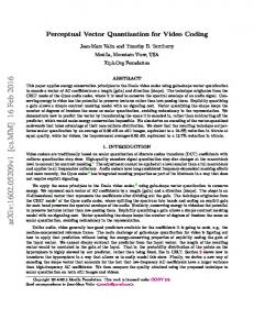
Fig. 1. THP system with Adaptive Vector Quantization. more efficient than transmitting the whole CIR parameters. The utilization of a static codebook is not adequate in our application because the quantizer will always apply the same fixed codebook ignoring that channels are time–varying. This limitation can be avoided if an Adaptive Vector Quantization (AVQ) is used for channel tracking. The appending of new vectors to the codebook is performed when the Euclidean distance between the new predicted channel realization and its nearest neighbor codebook vector is greater than some threshold value that determines the quantizer resolution. The least recently used codeword is then removed in order to maintain a constant codebook size. Thus, the codebook is refreshed dinamically according to the channel variations. Correspondingly, the modified codewords should be fed back to the transmitter only when significant changes have occurred. The remainder of this paper is organized as follows. In Section II, the signal model used along this work will be described. The adaptive vector quantization implemented by our precoding system will be briefly reviewed in Section III. Particle filtering techniques applied to obtain channel information at transmission are explained in Section IV. Finally, illustrative computer simulations are presented in Section V and some concluding remarks are made in Section VI. 2. SIGNAL MODEL Precoding techniques were first introduced separately by Tomlinson and Harashima in the early 1970’s [6, 7]. The principle of Tomlinson–Harashima Precoding (THP) can be !! MIMO channels as shown in [8, 9]. extended to ! Figure 1 shows the baseband representation of the signal model that will be used along this work. We will consider a digital communication system that sends BPSK symbols " !! ! " " #$#%, ! " $# ## % $ $ $, in frames of length
% & # through a MIMO frequency–selective fading channel. We will represent the channel by the !! ! & matrix !!,
!! "
! "
!
!
!!
.. .
"
.. .
!!
"!
&&& !
&&& !
!!
.. .
"! "
# $ %
(1)
!!
where the overall channel impulse response beetween the receiver antenna and the ( th transmit antenna is repre% sented by the vector #$ !! " ')!#$ !!# $ $ $ # )#$ !!℄, (' " ## %# $ $ $ # !! , ( " ## %# $ $ $ # ! ) and where & is the order of the finite impulse response (FIR) channel. Let us further elaborate our signal model by stacking the matrix !! into a column vector with ! !! & coefficients 'th
! !!
!
"
')
)
!
%
!! $ $ $ )!"!
!! $ $ $ )!" !! $ $ $ )!"! " !! $ $ $
%
% "
!! $ $ $ )"!
!! $ $ $ )
%
!! $ $ $ )"! " !!℄
&
(2) Throughout this paper we will assume that the elements !! are Gaussian random variables of the channel matrix with zero mean and unit variance. Consequently, the magnitudes of the channel gains ')'#$ !!', * " $# ## $ $ $ # & ( #, have a Rayleigh distribution, or equivalently expressed, ')'#$ !!'" are exponentially distributed. We will also assume that the channel gains are spatially uncorrelated. This model is known in the literature as uncorrelated Rayleigh MIMO channel. The channel time autocorrelation properties fit to the Wide-Sense Stationary and Uncorrelated Scattering model of Bello (WSSUS) [10], i.e.,
#
'
'
+ )#$ ! !)#$
!
%),
!" !
(
'
%-.) #$ % / !
(3)
where .) '#$ " .) is the Doppler frequency of the * * –tap between the ( th transmit antenna and the 'th receiver antenna, % is the duration of a frame, ,( is the zero-order Bessel function of the first kind and / " '! ( !" '.
A block fading channel is considered in which the CIR is constant for the duration of the frame and changes from one block to another according to a low order autoregressive process [11, 12] of order ,
!! "
!
!
!
"!
!
"! #
" !
" !!# !!
(4)
where !! is given by equation (2) and # !! is a zero– mean, i.i.d. and circular complex Gaussian vector process. Due to the WSSUS assumption, the !" !# # ! !" !# # matrices ! " ! are diagonal, being defined as ! " ! " $ " !", where $ " ! can be known a priori or estimated during an initial training period [13]. Model inaccuracies can be made arbitrarily small by increasing the order , although loworder autoregressive models are capable of effectively tracking the channel variations [11, 12]. If the !# –dimensional received signal is sampled at the symbol rate, we obtain the following discrete–time model,
$
!! " % !!
!! # & !!
(5)
where !! is given by equation (2), % !! is an input symbols matrix with size !# ! !# !" #, defined as
%
!!
"
!!"$ & & & %$! !!"$ & & & %! ! # # %!"$ & & & %$! !
$%!
# # %!"$
℄
(6) and & !! " $'! !! " " " '$ !!℄% is the zero mean spatio– temporally Additive White Gaussian Noise (AWGN) vector with variance (&" . If we employ the notation given by the equation (1), the received signal may be expressed as
$
!! " ' !!( !! # & !!
(7)
where ( !! is a !" # ! % vector defined as
(
!!
!!) & & & ) %! ! # # %!) & & & %$! !!) & & & ) %$! ! # # %!℄%
(8)
as you can see in figure 1. 2.1. Tomlinson–Harashima Precoding Design According to the discrete–time model given above, in order to calculate the optimum feedforward and feedback matrices when frequency–selective channels are considered, we define the z–transform of the channel matrix as
'
! "#
'
!
!
#
*! "
'!
!!* !
(9)
where the matrices '! !! will be given by
'!
!! "
+!!! !! .. .
+!$
! !!
""" .. .
"""
+!!$! !! .. .
+!$ $!
!!
$ %&
! !' * ! " )( * !!) * ! (11) ' ! ! where ) * ! will be given by ) * ! " ! # ) !!* ! . The time–domain matrix )! !! corresponding to ) * ! will be strictly causal (i.e., )! !! " *) " , (), minimum phase (i.e., )*+ ) * !! #" (, $* $ % %) and with the matrix )# !!
'(
'
*
lower triangular. For calculating ) * !, the first step is to express the product '( * ! !' * ! as
'(
*
!!' * ! " +( * ! # +# # +! * ! !
(12)
where +# and +! are constant matrices of dimensions !# ! !" . Then the Toeplitz matrix,
,"
( +#
+( ! +! +#
)
(13)
can be factorized by means of a Cholesky factorization as
)
(
, " !!( , where ! is expressed as ## * !" ! !!# !!! Therefore, the z–transform ) * ! will be obtained as ) !!! # !!# * !.
(14)
*! "
According to this spectral factorization, the feedforward matrix will be given as
-
* ! " )( *
! !'( * ! !
(15)
and the feedback matrix . * ! " can be obtained taking into account that . * ! is given by
$%!
"
Signal propagation studies show that the delay spread rarely exceeds of a few symbol periods in the cellular standards and, as a consequence, we will consider delays of only two time intervals, i.e., short channels with # " ' [12]. Designing Tomlinson-Harashima precoders for MIMO channels starts with the spectral factorization of
(10)
.
* ! " /) * !
(16)
where / is a !# ! !" matrix obtained from ) * ! by means of the inverse of the main diagonal of )# !!. The time– domain matrix .! !! corresponding to . * ! is thus strictly causal and minimum phase with .# !! unit–diagonal lower triangular (“monic” matrix polynomial . * !). For the details of this spectral factorization method see [14, 15]. In this paper we will assume that matrix F(z) is calculated from channel estimates obtained at the receiver. More specifically, we will explain in section 4 how to blindly estimate the channel by means of Sequential Importance Sampling (SIS) techniques which have the advantage of not requiring the transmission of pilot symbols. These channel estimates are applied to an adaptive vector quantizer to obtain the information to be transmitted through the feedback channel. The quantized channel estimates are then used to calculate matrix . * !.
3. ADAPTIVE VECTOR QUANTIZATION There are numerous algorithms for vector quantization. In this section we describe the algorithms that best fit to our application. We will start by presenting the mathematical preliminaries behind the theory of an adaptive vector quantizer [5]. 3.1. Mathematical definition of AVQ An adaptive vector quantizer, , is defined as a mapping at time ! from " –dimensional Euclidean space, ! , to a finite subset, ! , of ! , !
"# ! # ! $
!
$
(17)
The subset ! is called the codebook and is constituted by % codewords, " , i.e.,
!
!
% # ! # $ $ $ # # &#
'
"
!
$
(18)
Given an " –dimensional vector ! ' ! , the output of the vector quantizer is another " –dimensional vector, ! ", given by ! " ! "! ## ! " '!$ (19) Thus, for each time t, the vector quantizer divides the space ! into K partition regions, ( " , defined as
) & ) % (20) Each region is represented by a codeword from ! . From $ and ( " * this definition, it follows that " ( " ( % +, & , ' , so the set of ( " ’s form a partition of ( " %! ' !
$
!
"
# !
" &#
$
!
!
!
the space ! . Additionally, if the vector quantizer assigns a vector ! to the region ( " , ! is reproduced by the codeword " . In order to measure the difference between two vectors we have to define a vector distortion measure between an " ! "! #, i.e., input vector ! and its quantized version ! ("! # !" #. The most widely used measure of distortion is the squared error defined as
( ! # !" "
#
!
-! " !" -
!
! $
!
) ")
"
'"
'
" !"
!
! "
&
#
!
"
" !"
!
% '#
# !
(21)
An optimal vector quantizer for a given input random vector, !, will be the one that produces the smallest average distortion, i.e., produces the minimum mean squared error. 3.2. Communication System Model Using AVQ 3.2.1. Initial Codebook Design A fundamental problem when designing an AVQ is the obtention of the initial quantizer codebook. One of the most
useful and simple methods is termed pruning [5]. With this technique, we start from a training data sequence and selectively eliminate training vectors as candidate codewords until a final set remains as the codebook. In other words, at the beginning, we put the first training vector in the codebook. In the sequel, a training vector will be added to the codebook only if the distance between that vector and its nearest neighbor (21) is greater than some threshold *. Otherwise, the corresponding training vector will be rejected. If the resulting codebook has less than the desired number of codevectors the threshold value must be reduced and the process repeated again. The quality of this initial codebook can be considerably improved by means of the Lloyd algorithm. More specifically, we focus on the Generalized Lloyd Algorithm (GLA) because it is the most widely used in the literature. GLA is an extension to vector quantization of the original Lloyd algorithm, although is commonly known as LBG algorithm due to the paper of Linde et al. [16]. GLA consists of alternatively applying the nearest–neighbor and centroid conditions [5] to yield smaller average distortion. An adequate initial codebook choice is very important to get optimal convergence in GLA. 3.2.2. AVQ Algorithm Contrary to conventional VQ, adaptive VQ algorithms allow the codebook to be modified while the data transmission process is in progress. This is important in our work since we are interested in quantizing MIMO channels that are time–varying. Among the different adaptive VQ algorithms proposed in the literature, we have selected the Paul algorithm [17, 18] due to its adequate compromise between complexity and performance. In the Paul algorithm we start by finding in ! ! the codeword " that is closest to the current channel vector ! . If the distance between the that vector and its closest codeword is less than the distortion threshold, i.e., &'(
( ! # ) *# "
"#
$
)&)%
(22)
the index of this codeword will be sent to the transmitter. We also transmit an one–bit flag as side information to indicate that we are not updating the codebook. We then set ! ! ! ! and repeat the process for the next vector. If the distortion between the closest codeword and the current channel vector is greater than the distortion threshold, i.e., &'(
( ! # + *# "
"#
$
)&)%
(23)
we update the codebook. In this case, we form ! by replacing the Least–Recently–Used (LRU) codeword of ! ! with the current vector. As side information, we will send the new codeword to the transmitter, as well as an one–bit
flag indicating that we are updating the codeword. We also transmit the index of the LRU codeword to the transmitter to reduce searching time at transmission. Therefore, the Paul algorithm ensures that each channel vector is coded with a distortion which is, at most, the value of distortion threshold . Notice that the Paul algorithm can update the codebook for each new channel realization. Consequently, it can adapt very quickly to abrupt changes in the channel statistics. However, the amount of side information sent to the transmitter could be quite substantial, as we will have to send the new codewords to the transmitter for each update. The original Paul algorithm used a fixed–length index encoder. The overhead could be reduced by using variable– length coding. Nevertheless, if we use a variation of the Paul algorithm introduced by Goodman et al. [19], feedback rates will be even lower [18]. This technique, known as the move–to–front algorithm, involves “rearranging” the codewords and “reassigning” its index during the encoding process. If the codebook is not updated, after the index of the closest codeword is sent to the transmitter, that codeword is simply moved to the front (index number 1) of the codebook in both the transmitter and the receiver. Otherwise, if the codebook is updated, the new codeword is added to the beginning of the codebook and the index of each of the remaining codewords is incremented. The last codeword in the codebook will be deleted. Therefore, this scheme has the additional advantage that, since both transmitter and receiver know where to put the new codeword, transmission of an index specifying the point of insertion of that codeword is not needed. Since codewords that are more frequent tend to be assigned small index values, feedback rate will be decreased when variable–length index coding is applied.
4.1. SIR Algorithm with Known Channel Order In Importance Sampling (IS) [21], we assume that ! particles from a trial probability mass function (p.m.f.) are drawn and weighted according to the true posterior probability of the data sequence conditioned on the corresponding series of observations " # ! $ ! ℄, i.e, "!# # !
Kalman filtering is the most widely used method for estimating and predicting the CIR of a time–varying channel. Nevertheless, it is important to note that Kalman filtering is a supervised method that estimates the channel only during the time intervals where pilot symbols are transmitted. On the other hand, there exist blind methods that do not need explicit knowledge of the transmitted symbols and thus can track channel variations continuously during the transmission of information data. This approach reduces overheads in transmission and increases the spectral efficiency of the communications link. Particle filtering techinques, such as Sequential Importance Resampling (SIR) [20], are an example of blind approaches to the estimation of time–varying channels.
%# !
$ !
(24)
℄
where # ! " "# & #$ & ' ' ' & # # are the symbols transmitted in a single frame and % # ! $ ! ℄ is the trial or importance probability mass function (p.m.f.) with the same support as " # ! $ ! ℄ but easier to sample. The normalized importance weights "("!# #!%$"###"$ are defined as ( #
"!#
("!#
"!# "# ! $ ! "!# %# ! $ !
"
"
℄
(25)
℄
"!# ( #
(26)
$ "%# # %%$ (
The particles and their weights provide a Monte Carlo estimate of the true posterior p.m.f., "# !
$ !
℄ $ " $
# !
$ !
℄ "
$ ! !%$
Æ! (
"!#
(27)
"!#
where Æ! " % if # ! " # ! and Æ! " & otherwise. The IS method can be modified so that it becomes possible to build "!# the state trajectories # ! and the importance weights ("!# sequentially as new observations arrive. Let us consider the following factorization of the importance p.m.f. % # !& $ !& ℄
4. CHANNEL TRACKING
!
%
% #& # !& $ & $ !& ℄% # !& $ $ !& $ ℄&
&*'
(28) Dealing with (28), the IS principle and the following descomposition of the posterior p.m.f., " # !& $ !& ℄
" $& # !& & $ !& $ ℄" # !& $ $ !& $ ℄
%
(29)
it is simple to see that the importance weights can be evaluated recursively in time, leading to the Sequential Importance Sampling (SIS) algorithm "!# #&
( #
"!#
"
"!# % #& # ! & $ & $ ! & ℄
(30)
"!# "!# " $& # !& & $ !& $ ℄ (& $ "!# "!# % #& # !& $ & $ !& ℄
(31)
%
"!# (&
"
"!# ( #&
"%# $ #& %%$ (
(32)
for !! " " " ! # . The set of particles and normalized weights at time t, !
! " $% !
!
$"#! ! %!
(33)
is a discrete random measure that yields to a MC estimate of the posterior p.m.f. analogous to equation (27),
"
& $"#! "'"#!
℄ # &$"$
"
"#! '"#!
"
℄
Æ %!
!
(34)
%$It can be shown that &$"$"#! "'"#! ℄ converges to &"$"#! "'"#! ℄ as # $ % . At time t, the particle smoother can be used to extract estimators from the posterior distribution. For example, the #$ MAP estimate of the state sequence, $" , can be appro"#! ximated by the particle with the largest importance weight, i.e., ! ) $""#!#$ % $"#%&' (35) !
!! & & & ! # . where %&' $*+ &'( %! !! It is shown that if the channel order is known, as in our case, the CIR vector has a prior Gaussian distribution, !
" ℄
&
' )!
!
*
"
(36)
where ! and " are the a priori channel mean and covariance matrix, respectively. Then, the posterior channel probability density function (p.d.f.) given a sequence of observations, '"#! , and transmitted symbols, $"#! , is also Gaussian, i.e., &" "$"#! ! '"#! ℄ ' ) ! ! ! "! * (37) and the distribution parameters can be updated recursively according to
"! % !!
! " !
(
$! $! ,& )
$! '! & ,)
+"
!
% %
% ! %
!!
+"
#
%
"
(38) (39)
$
The posterior channel distribution associated to the hi! ! ghest importance weighted particle ' !! !" ! "! !" , provides a Bayesian estimate of the CIR. 4.1.1. Resampling A major problem with particle filtering is that all the particles, except for a very few, are assigned negligible weights. This degeneracy implies that the performance of the particle filter will deteriorate. One approach to alleviate this problem [22, 23] is to include a resampling step in the SIS algorithm [22]. Intuitively, the resampling operation consists of discarding those state trajectories with very small importance weights, while those with a higher probability are replicated. As a result, the recursive method Sequential Importance sampling with Resampling is obtained [22].
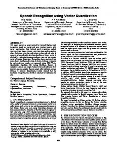
5. RESULTS We carried out computer experiments to illustrate the feasibility of an adaptive MIMO transmission system with Tomlinson-Harashima precoding that estimates the channel using SIR techniques and quantizes the estimates with AVQ. In spite of prediction and quantization errors simulations show that degradation in performance when transmitting BPSK constellation points over spatially uncorrelated MIMO Rayleigh fading channels is acceptable. -* , MIMO system with Let us consider a -! Zero Forcing TH precoding. We modeled channel variations as an ./)!* aproximation according to Bello’s model. The AR coefficient is a function of the Doppler spread. To estimate the bit error rate having into account this channel model, ,--- data frames of size .- (i.e. 100,000 bits) have been randomly generated. The channel will be constant across a data frame and changes according to the model explained in Section II from one block to another. The SIR algorithm is evaluated with 0 ,-- particles. With & ,) being the noise variance, the SNR plotted is given by 10 / !-23+4( 5,)& , where 4( is the transmit power in each slot. Figure 2 presents the estimated BER curves for a normalized Doppler frequency 6+ 7 -"-,, i.e., relatively fast fading channel. The figure shows the large loss in performance when the predicted channel is employed at transmission caused by prediction errors. However, the mismatch beetween the true channel and the predicted one is compensated by means of a linear adaptive residual equalization at the receiver side. From the figure, it can be seen too how the use of precoding techniques is advantageous over the simple linear equalization at the receiver. Figure 3 plots the precoding performance for 6+ 7 -"-, when adaptive vector quantization is applied in order to limit the feedback ratio. The picture plots the BER for three different values of the threshold parameter 8. If 8 is too large, the performance will be strongly degradated, but if the choice of this parameter is suitable, AVQ will correctly track the channel time variations even when the predicted channel is employed in the precoder design, as shown in the figure 3. Therefore, the optimal value of 8 must be modified depending on the fading speed during the initial training period where the codebook is generated to ensure a good performance and optimal compression ratio. The selection of the codebook size however is not so critical in terms of BER performance and compression ratio. The following tables illustrate quite clearly the compression ratios for the feedback channel when AVQ is employed. In table 1 it can be seen compression ratios when the parameter 8 adopts different values. Obviously, larger values of 8 yield to larger ratios at the cost of decreasing performance, as shown in
0
0
10
10 Perfect CSI Imperfect CSI/ZF−LE Imperfect CSI No precoding/ZF−LE
No AVQ AVQ (0.001) AVQ (0.01) AVQ (0.1) −1
10 −1
10
−2
BER
BER
10 −2
10
−3
10
−3
10
−4
10
−4
10
0
5
10
15 SNR(dB)
20
25
30
0
5
10
15 SNR(dB)
20
25
Fig. 2. Precoding performance vs. SNR.
Fig. 3. Precoding performance vs. SNR using AVQ.
figure 3. In table 2, compression ratios depending on the codebook size obtained also via computer simulations are presented. For reasonable codebook sizes high compression ratios could be achieved, while increasing codebook size indefinitely does not involve a significant improvement in terms of performance. Nevertheless, larger codebook sizes imply that more storage capabilities will be needed at the receiver.
6. CONCLUSIONS
0.001 0.005 0.01 0.05 0.1
Compression ratio 4.12 10.34 12.25 17.37 19.20
[1] G. Foschini and M. Gans, “On limits of wireless communication in a fading environment when using multiple antennas”, Wireless Personal Communications, pp. 311-335, March 1998. [2] L. Hanzo, C. H. Wong and R. M. S. Yee, Adaptive Wireless Transceivers, John Wiley & Sons Ltd, 2002.
Compression ratio 4.92 7.09 9.11 12.25 12.28 12.29 12.64 13.80
Table 2. Compression ratio vs. codebook size for
In this paper we have demonstrated the feasibily of Adaptive Vector Quantization (AVQ) for implementing Tomlinson–Harashima precoding MIMO techniques. We have also considered the effect of estimating the channel using a blind method such as Sequential Importance Resampling (SIR). Thanks to AVQ, the feedback channel overhead is strongly reduced with a small loss in performance. Thus, we are capable of adapting the precoder to channel variations with a limited feedback channel. 7. REFERENCES
Table 1. Compression ratio vs. threshold parameter . Codebook size 4 8 16 32 64 128 256 1024
30
[3] R. F. H. Fischer, Precoding and Signal Shaping for Digital Transmission, John Wiley & Sons, Inc., Publication, New York, 2002. [4] David J. Love, Robert W. Heath Jr., Wiroonsak Santipach and Michael L. Honig, “What is the value of the limited feedback for MIMO channels?”, IEEE Communications Magazine, pp. 54-59, October 2004.
!!!".
[5] A. Gersho and R. Gray, Vector Quantization and Signal Compression, Kluwer Academic Publishers, 1992.
[6] M. Tomlinson, “New Automatic Equalizer Employing Modulo Arithmetic”, Electronic Letters, pp. 138-139, March 1971.
[15] V. Kuˇcera, “Factorization of Rational Matrices: A Survey of Methods”, Proc. IEE Intern. Conference on Control, pp. 1074-1078, Edinburgh, 1991.
[7] H. Harashima and H. Miyakawa, “Matched–Transmission Technique for Channels with Intersymbol Interference”, IEEE Journal on Communications, pp. 774780, August 1972.
[16] Y. Linde, A. Buzo, and R. M. Gray. “An algorithm for vector quantizer design”, IEEE Trans. Comm., COM– 26:702-710, April 1978.
[8] Robert F.H. Fischer, Christoph WindPassinger, Alexander Lampe and Johannes B. Huber, “Space–Time Transmission using Tomlinson–Harashima Precoding”, in 4th International ITG Conference on Source and Channel Coding, Berlin, January 2002. [9] Robert F.H. Fischer, et al., “MIMO precoding for decentralized receivers”, in Proc. of ISIT’02, Lausanne, Switzerland, June/July 2002, p. 496. [10] P. A. Bello, “Characterization of Randomly Time– Variant Linear Channels”, IEEE Trans. on Communications Systems, vol. CS-11, pp. 360-393, December 1963. [11] C. Komninakis, C. Fragouli, A. H. Sayed and R. D. Wesel, “Multi-Input Multi-Output Fading Channel Tracking and Equalization Using Kalman Estimation”, IEEE Trans. on Signal Processing, vol. 50, nÆ 5, May 2002. [12] C. Komninakis, C. Fragouli, A. H. Sayed and R. D. Wesel, “Channel estimation and equalization in fading”, Signals, Systems, and Computers, 1999. Conference Record of the Thirty-Third Asilomar Conference on, vol. 2, pp. 1159-1163, October 1999. [13] M. K. Tsatsanis, G. B. Giannakis and G. Zhou, “Estimation and Equalization of Fading Channels with Random Coefficients”, Signal Processing, vol. 53, pp. 211229, 1996. [14] D. C. Youla, “On the factorization of rational matrices”, IRE Trans. on Information Theory, vol. IT-7, pp. 172-189, Jul 1961.
[17] D. B. Paul, “A 500-800 bps adaptive vector quantization vocoder using a perceptually motivated distance measure”, in Conf. Rec. IEEE Globecom, 1982, pp. 1079-1082. [18] J. E. Fowler, Adaptive Vector Quantization for the Coding of Nonstationary Sources, Ph.D. dissertation, The Ohio State University, 1996. [19] R. M. Goodman, B. Gupta, and M. Sayano, ”Neural network implementation of adaptive vector quantization for image compression”, Tech. Rep. Department of Electrical Engineering, California Inst. Technol., Pasadena, CA, 1991. [20] J. M´ıguez and P. Djuric, “Blind Equalization of Frequency-Selective Channels by Sequential Importance Sampling”, in IEEE Transactions on Signal Processing, vol. 52, no. 10, pp. 2738- 2748, October 2004. [21] J. Geweke, “Bayesian inference in econometric models using Monte Carlo integration”, Econometrica, vol. 24, pp. 1317-1399, 1989. [22] A. Doucet, S. Godsill and C. Andrieu, “On sequential Monte Carlo Sampling methods for Bayesian filtering”, Statistics and Computing, vol. 10, no. 3, pp. 197-208, 2000. [23] A. Kong, J.S. Liu and W.H. Wong, “Sequential imputations and Bayesian missing data problems”, Journal of the American Statistical Association, vol. 9, pp. 278288, 1994.